Basic Concepts in Probability and Information Theory
This lecture summarizes basic terminology and concepts in statistics and probabilities and how they can
be applied to model a specific linguistic task: parts of speech tagging.
The following notes from this course introduce terminology in a concise and useful manner:
Statistical Methods for NLP, Goteborg's University:
- Probability Theory
- Random Variables
- Information Theory
- Statistical Inference
- Markov Models
- Parts of Speech Tagging: Statistical Models
Other excellent tutorials on Machine Learning are available in repository of tutorials
by Andrew Moore (Carnegie Mellon University) (also available here).
In particular, read:
- Probabilistic and Bayesian Analytics
- Cross-validation for detecting and preventing overfitting
The following article: An Intuitive Explanation of Bayes' Theorem, by Eliezer Yudkowsky, provides a humourous and useful introduction to
Bayesian reasoning that you may find useful.
In the following, we summarize Chapter 1 of Pattern Recognition and Machine Learning by Chris Bishop to get an
operational feeling of how probabilities, information theory and decision theory help us design computational models of machine learning.
Probability Theory
Probability theory allows us to infer quantified relations among events in models that capture uncertainty in a rational manner.
A probability function assigns a level of confidence to "events". The axiomatic formulation includes simple rules. Consider we
are running an experiment, and this experiment can have n distint outcomes. We want to be able to discuss our level of certainty
about the results of the experiment.
Consider the set Ω of outcomes. An event is defined as a subset of outcomes from Ω -- there are 2n events over Ω.
Define a function p that meets the following conditions:
p: 2Ω → [0..1] (that is, for all event e, 0 ≤ p(e) ≤ 1)
p(A ∪ B) = p(A) + p(B) - p(A ∩ B)
p(∅) = 0
p(Ω) = 1
Random Variables
We map the presentation of uncertainty in terms of outcomes and events
to that of random variable. The value of a random variable
corresponds to the possible outcomes of the experiment. We will
consider real-valued random variables. In NLP, we will often consider
random variables representing the experiment of choosing a word within
a vocabulary or choosing a sentence within a language. In this case,
the random word is modeled as the index of the word within the
vocabulary of possible words. We will often use an alternative model
using an indicator vector, which is a vector of boolean values
(0 or 1) of dimension N = size of the vocabulary and in which exactly
one element is 1 and all the others are 0, with the 1 appearing at the
position of the selected word into a vocabulary. A "random sentence"
may be parameterized as a vector of random words.
The computations predicted by probabilities become interesting and sometimes
surprising when we consider complex experiments, involving multiple random variables.
The dependency relations among the variables are reflected in the computations using
simple rules -- called "sum and product rules of probability".
Consider the classical example of boxes and balls with Bishop's figure:
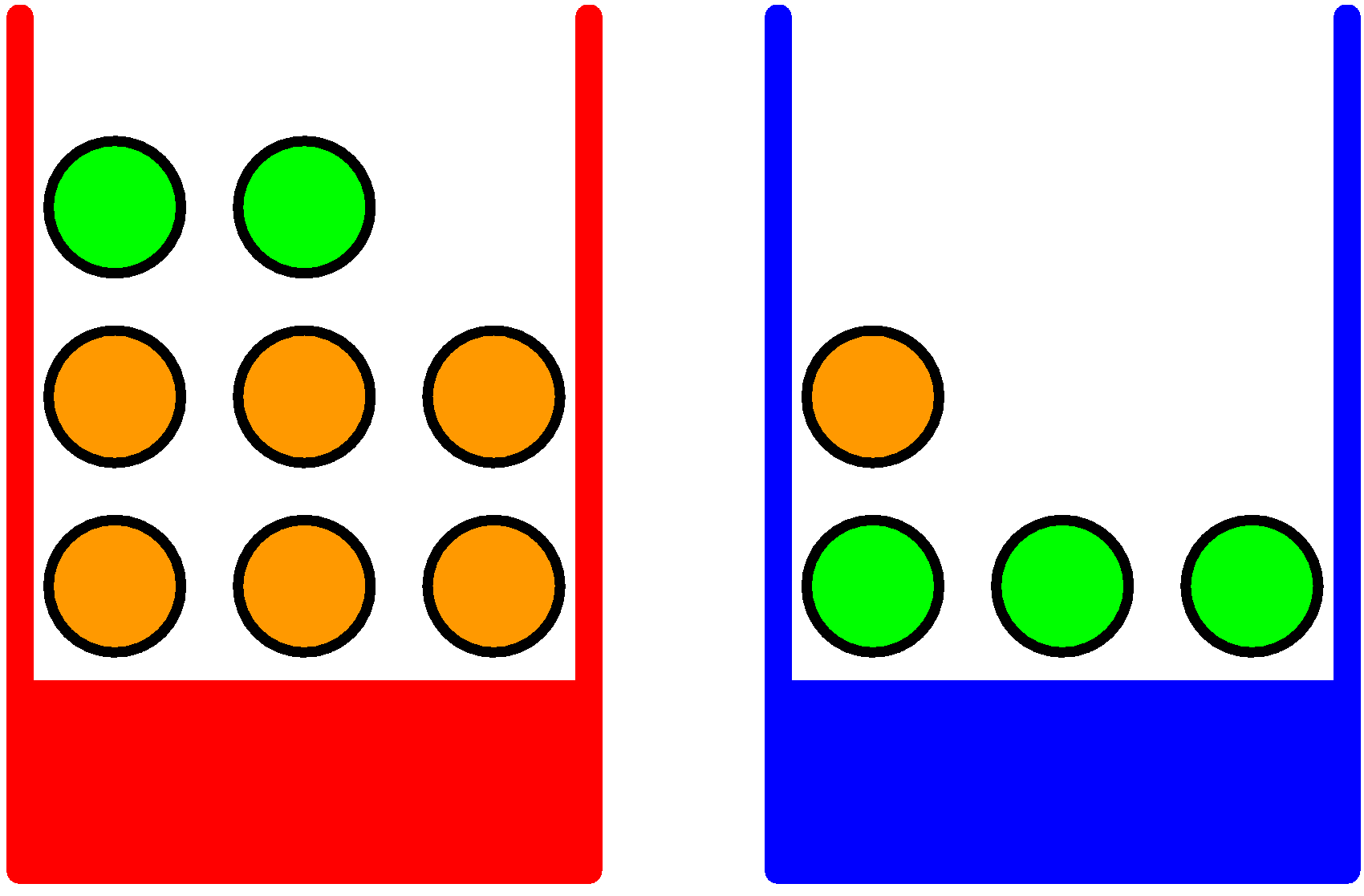 In this setting, we are considering a "structured experiment" which
proceeds in 2 stages: first pick a box (either red or blue), then pick
a ball within the selected box (either orange or green).
Assume we repeat this experiment many times, and assume we get the following aggregated observations:
In this setting, we are considering a "structured experiment" which
proceeds in 2 stages: first pick a box (either red or blue), then pick
a ball within the selected box (either orange or green).
Assume we repeat this experiment many times, and assume we get the following aggregated observations:
- p(red box) = 40%
- p(blue box) = 60%
- All balls in the box are equi-probable (can be picked equally likely)
We model this experiment with 2 random variables:
- B ∈ {blue, red} (the box can be either blue or red)
- F ∈ {orange, green} (the ball can be either orange or green)
When we consider 2 variables, we can think of the outcomes of the experiment as a matrix, where the cells
measure the number of outcomes for the joint occurrence of each of the variables, as illustrated here:
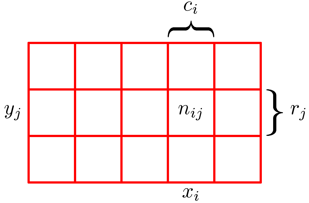 In this view, we can define several interesting quantities (assuming we ran the experiment N times, and N → ∞):
- p(X = xi, Y = yj) = nij/N is the joint probability
- p(X = xi) = Σj p(X = xi, Y = yj) = ci/N is the marginal probability
- p(X = xi | Y = yj) = nij / yj is the conditional probability (read as probability of X=xi given that Y=yj)
From these definitions, we derive that:
p(X = xi, Y = yj) = p(Y = yj | X = xi)p(X = xi)
p(X = xi, Y = yj) = p(X = xi | Y = yj)p(Y = yj)
and in general, the following relation known as Bayes rule:
p(Y | X) = p(X | Y) p(Y) / p(X)
p(X) = ΣYp(X|Y)p(Y)
These simple rules can provide interesting results - as applied to our box and balls example:
p(B = r) = 4/10
p(B = b) = 6/10

p(F = g | B = r) = 1/4
p(F = o | B = r) = 3/4

p(F = g | B = b) = 3/4
p(F = o | B = b) = 1/4
We can now compute the probability that a ball is orange or green based on the complex experiment:
p(F = o) = p(F = o | B = r)p(B = r) + p(F = o | B = b)p(B = b) = 9/20 = 0.45
p(F = g) = 11/20 = 0.55
Compare this result with the uniform probability we would obtain if we ignore the structure of the boxes:
there are overall 7 orange balls and 5 green balls. The uniform probabilities would have been
p(F = o) = 7/12 = 0.58 -- because the boxes introduce structure over the balls, they significantly affect
the likelihood of picking an orange or a green ball (p(o) changes from 0.58 to 0.45).
Another non-trivial computation is obtained by applying Bayes rule. Bayes rule in general is used to "reverse dependency".
Consider the following observation: we run the experiment and we obtain an orange ball. What is the likelihood that the ball
was picked from the red box?
p(B = r | F = o) = p(F = o | B = r)p(B = r)/p(F = o) = 2/3
One way to read this result is as follows: if we do not have any
additional data, then the probability that the red box has been picked
is 40%. But if we are told that an orange ball has been picked, then
we can revise our estimation -- and we can now believe that the red
box has been picked with 67% confidence. That is, we updated our
confidence because we were given additional data - from 40% to 67%.
You can solve the example given in the article quoted above: An Intuitive Explanation of
Bayes' Theorem using this formula:
1% of women at age forty who participate in routine screening have
breast cancer. 80% of women with breast cancer will get positive
mammographies. 9.6% of women without breast cancer will also get
positive mammographies. A woman in this age group had a positive
mammography in a routine screening. What is the probability that she
actually has breast cancer?
The solution is 7.76% -- which is quite not intuitive even on a very
simple binary case. Make sure to work out the formula to convince yourself
of how the result is obtained.
Independence
We say that two random variables are independent if the following relation holds:
p(X,Y) = p(X)p(Y)
In terms of information obtained by running an experiment, independence means that knowing the value of Y
does not reduce the uncertainty about X. Another way to look at independence is to use the notion of
conditional probability.
In general:
p(X, Y) = p(X | Y) p(Y)

When X and Y are independent, then:
p(X, Y) = p(X | Y) p(Y) = p(X) p(Y)

Hence:
p(X | Y) = p(X)
That is, the fact that Y is given does not change the uncertainty on X.
We can extend the independence relation to conditional independence:
X and Y are conditionally independent in Z iff:
p(X,Y|Z) = p(X|Z)p(Y|Z)
Continuous case: Probability densities
So far we worked over a discrete set of events over a discrete set of outcomes Ω.
Probability functions can be extended over continuous variables (real numbers). In this case,
we will move from discrete sums (Σ) to integrals and the probability function is defined
in terms of a probability density function (pdf) p such that:
p(x ∈ [a..b]) = ∫ab p(x)dx
The normalization condition on a pdf is:
∀ x, p(x) ≥ 0
∫-∞+∞ p(x)dx = 1
We extend the definition of pdfs to multiple variables and the marginal and conditional probabilities
as follows:
p(x) = ∫ p(x,y)dy
p(x,y) = p(y|x)p(x)
Expectation and covariance
Given a probability function, we can use it to compute the weighted average of a function.
In this case, we use the terminology of a probability distribution p(x) which determines
how likely each value of x is over a range of possible values. We can then define the expectation of f relative to p
as:
Ex(f) = Σx p(x)f(x)  for the discrete case
Ex(f) = ∫x p(x)f(x)dx  for the continuous case
An important operation over a probability distribution is that
of sampling: sampling is the operation of randomly choosing a
value x out of the range of values which x can take so that if we keep
sampling many times (N), we observe each value x about p(x).N times out
of N.
If we sample x many times and obtain values (x1...xN), then the following approximation holds:
E(f) ≅ 1/N Σn=1Nf(xn)
Expectation can also be extended to multiple variables, with the expected generalization for conditional expectation:
Ex[f(x,y)] = Σxf(x,y)  (This is a function of y)
Ex[f | y] = Σx p(x | y) f(x)
The variance of f is defined as:
var(f) = E[(f(x) - E(f(x)))2] = E[f(x)2] - E[f(x)]2
Similarly, the variance can be extended to multiple variables, and we obtain the definition of covariance:
cov[x,y] = Ex,y[{x - E(x)}{y - E(y)}] = Ex,y[xy] - E[x]E[y]
Variance is the special case of cov(x,x).
Expectation and variance are useful summaries of a complex probability distribution -- they tell us in 2 numbers something
useful about a full distribution -- what is the mean value and how much variability there is around the mean. Often, we want
to model the following situation: we know that a quantity has been measured with some level of noise; in such a case, we are
looking for a way to describe what we know about the quantity. One way is to state that the actual quantity has a certain expected
value (derived from the measurement) with some level of variance (corresponding to the accuracy of the measurement method).
In this case, the 2 quantities that characterize the possible distribution of the quantity are its expectation and its variance.
If we know more about the measurement process, we can suggest a finer distribution model. Otherwise, we use a standard distribution
model (typically, we use the Gaussian distribution in such cases as described below).
In the case of two variables, covariance is a measure of how much two
random variables change together. For example, if in general we
observe that when x grows, then y tends to grow as well, and when x
decreases, then y decreases as well, that is, x and y show in general
a similar pattern, then the covariance is positive. If the behavior
is inverse, that is, when x grows, y decreases and vice versa, then
the covariance is negative. If there is no correlation between x and
y (they are independent), then the covariance is 0. The
interpretation of the magnitude of the covariance is not easily
interpreted.
What can be done with a distribution
Consider a distribution as an "object" in a programming language. What interface should the distribution object implement?
In other words, what are the useful operations one can perform on a distribution?
The following are the key operations:
- Sample: draw a random value from the distribution, such that, if we keep sampling many times, the sampled objects are distributed as predicted by the distribution.
- Estimate: given a set of samples, guess which distribution is likely to have generated these samples. Estimation is the reverse operation of sampling. We can think of it as a "factory method".
- Marginalize: given a joint distribution p(x,y), compute the marginal distribution p(x) or p(y)
- Condition: given a joint distribution p(x, y), compute the conditional distribution p(x|y) or p(y|x)
- Expectation: compute the expectation of the distribution Ep(x) - think of it as the weighted average of the distribution
- Variance: compute the variance of the distribution - think of it as the measure of variation around the average
- Average: given a function f, compute the weighted average of the function over the distribution, that is Ep(f(x))
These operations are the key ingredients used by machine learning
methods. They can be combined in many ways to solve problems of
regression (guessing a continuous function given samples of the
form (input, target)) and classification (guessing a discrete
function mapping input values to discrete classes given a set of examples.
When X is drawn from a distribution D, we note:
X ~ D
We will use this notation extensively to describe hierarchical distribution models.
Likelihood and Maximum Likelihood Estimation
The basic method of estimation is based on Bayes theorem:
p(w|D) = p(D|w)p(w)/p(D)
Consider a distribution p, characterized by parameters w. We are
interested in estimating the parameters w given an observed dataset D.
In the Bayes equation, we use the following terminology:
- Posterior: p(w|D) is the updated distribution over w given the observation D (that is, it reflects what we know about w after we have observed D).
- Prior: p(w) is the distribution over w independently of observations (that is, it reflects what we know about the parameters independently of any observation).
- Likelihood: p(D|w) is considered as a function over w, it reflects how likely it is that we sampled the dataset D from the distribution given a value of w.
Note that the likelihood as a function of w is NOT a distribution over w (that is, there is no normalization constraint that the sum of the likelihood for all possible values of w be 1).
Given this terminology, we restate that Bayes theorem as:
posterior ∝ likelihood x prior
Not that we "hide" the normalizing term p(D) which is a constant in w in the "proportional" sign.
If we were interested in computing p(D), we would use the following approach:
p(D) = ∫ p(D|w)p(w)dw
(Remember in the case of the mammography diagnostic example above, the computation of p(D) was quite important.)
The frequentist approach to estimation consists in finding the best
possible value for w given an observation D. In this case, the
normalization constant p(D) plays no role, and the output is an
optimal value for w, w*. That is, w* is a pointwise estimate of the distribution parameter.
The Bayesian approach instead tries to estimate
the distribution over w, p(w|D). This requires the computation of the
normalization constant p(D).
In general, Bayesian approaches to estimation are most useful if the task
we perform (regression or classification) is one step within a multi-step
process. The Bayesian approach is preferable in this case because the output
of the classification for example, does not need to choose the most likely
value for w, but instead can let further steps choose among multiple options
that may be likely and can be determined based on features which are not
considered at the time of the classification. For example, consider the task
of syntactic parsing. Parsing often uses as features the parts of speech of each
word. Therefore, the classification task of parts of speech tagging is one step
in the 2-step process of parsing. The frequentist approach will compute the most
likely POS tag for each word before parsing starts. The Bayesian approach will
instead compute a distribution over possible POS tags for each word, which can be
later used by the parser.
Estimation can proceed in 3 different ways, of increasing complexity:
- Maximum likelihood: find the parameter w* which yields the
maximum likelihood. w* = argmax p(D|w). This ignores the prior term
p(w) and the normalization constant p(D) in Bayes's equation. Maximum
likelihood estimators have a tendency to over-fit the data.
- Maximum a posteriori estimate (MAP): this method tries to
maximize the likelihood together with a prior: find the parameter w*
which yields the maximum value for the composed term likelihood x
prior, assuming a given prior distribution over w. w* = argmax
p(D|w)p(w). This has the effect of avoiding overfitting and is
similar to regularization. This ignores the normalization constant
p(D) in the Bayes equation.
- Bayesian estimation: find the posterior distribution p(w|D)
by computing the full right-hand side of Bayes equation. p(w|D) =
p(D|w)p(w)/∫ p(D|w)p(w)dw. This is the most
informative way to estimate, but is computationally expensive.
We will now illustrate these estimation methods on well known distributions.
Useful Distributions
A small set of simple probability distributions play a central role in probability theory. They are useful because they
can be used as building blocks to construct more complex distributions in a modular manner. We review 3 such distributions here:
Bernouilli, multinomial and normal (or Gaussian) distributions. These distributions are all characterized by a small set of parameters
and one can think of our work in the following as designing a basis to describe many useful distributions by combining simple basic distributions
each with its own parameters.
When solving a supervised machine learning problem, we attempt to
characterize the distribution of a random variable (the value to
predict) given a set of examples (observations). One way to
characterize this operation is as an operation of estimation of the
parameters of a distribution from a known family given the
observations. We will, therefore, often end up performing continuous
parameter estimation (and use integrals) to learn a function that maps
input parameters to predicted values on the basis of discrete
examples.
Bernouilli binary distribution
The Bernouilli distribution models the simplest experiment one can think of: throw a random coin and record the outcome as either 0 or 1.
The distribution is characterized by a parameter μ which is the probability of obtaining 1:
p(x=1|μ)=μ  where 0 ≤ μ ≤ 1
p(x=0|μ)=1-μ
We will summarize these 2 terms with a single expression, which will be useful to formulate sums and expectations over the Bernouilli distribution:
Bern(x|μ)=μx(1-μ)(1-x)
We can then verify that:
E(p) = μ
var(p) = μ(1-μ)
Consider a dataset of N observations drawn independently from the Bernouilli distribution D=(x1...xN), then
we can consider the likelihood of this dataset, which we consider as a function of μ for D given:
Computing the maximum likelihood estimate of a Bernouilli distribution
Given D = (x1...xN):
p(D|μ) = ∏n=1Np(xn|μ) = ∏ μxn(1-μ)(1-xn)
We derive this expression from the fact that the observations are
independent of each other (hence the product).
In order to derive the maximum likelihood estimate μML, we most solve:
μML = argmaxμ p(D|μ)
To obtain the maximum of the likelihood function, we must compute its derivation.
It is unpleasant to derive long products, so instead, we will look for the maximum
of the log-likelihood function. The log likelihood is:
ln p(D|μ) = Σ ln p(xn|μ) = Σ {xnlnμ + (1-xn)ln(1-μ)}
We take advantage of two properties of the log function here:
- Log is a monotonic function - and therefore, argmax(log(f)) = argmax(f)
- Log(axb) = Log(a) + Log(b) (and hence Log(an) = nLog(a))
Remember also that d ln(x)/dx = 1/x.
By computing the derivation of the log likelihood as a function of μ,
we derive that the likelihood reaches its maximum on:
d LogLikelihood(μ) / dμ = Σ {xn/μ - (1-xn)/(1-μ)}
μML = 1/N Σ xn
Another advantage of logs is that they avoid the problem of floating point underflow.
When we implement numerical algorithms involving probabilities, we have to deal with very small quantities (p(x) is a number between 0 and 1).
When we multiply small floating point numbers, we quickly reach a situation of numerical underflow, and the result is approximated to 0.
To avoid this, we perform computations on logs of probabilities, and add these logs instead of multiplying the probabilities.
With a dataset D=(x1...xN), we assume that for all i in (1..N), xi ~ Bernouilli(μ)
and we say that the N variables xi are independent and identically distributed (IID).
As as typical for MLE (maximum likelihood estimates), this MLE estimate severely overfits the distribution when the dataset is small.
Binomial Distribution
A close variant of the Bernouilli distribution is called the
binomial distribution: it describes the distribution of the
number m of observations of x=1 of a Bernouilli experiment repeated N
times. A binomial distribution has 2 parameters: μ is the
parameter of each Bernouilli draw and N, the number of repetitions.
Since the N draws are independent of each other, we derive that:
Bin(m|N,μ) ∝ μm(1-μ)N-m
To normalize this (that is, to make sure that the sum of Bin(m) over all possible m values from 0 to N is equal to 1), we must count all the distinct ways to obtain
m draws of 1s out of N draws. This number is (N choose m) noted (N m) = N!/(N-m)!m!
We derive the following properties for the binomial distribution:
Bin(m|N,μ) = (N m) μm(1-μ)N-m

E[m] = Nμ
var[m] = Nμ(1-μ)
Exercise: Compute the MLE estimator μMLE of a binomial distribution Bin(m|N, μ).
Choosing a Prior for the Binomial Distribution
If we want to compute a Bayesian estimate of Binomial experiments, we must select a prior for the distribution of the parameter μ.
We choose this in a way that is intuitively appealing (we can say something understandable about the expected value of μ and its variance)
and analytically convenient (we can easily integrate the prior).
To this end, note that the likelihood function of the Bernouilli distribution has a form which is proportional to μx(1-μ)1-x.
If we choose the prior to also be a power of μ and (1-μ), then the posterior distribution will also have the same form as the prior. This is convenient
because it means the posterior distribution will belong to the same family of functions as the prior, and the Bayesian update procedure will consist of only
updating the parameters of the prior distribution. This convenient property is called conjugacy: we identify the conjugate prior of the binomial distribution
to be:
Beta(μ|a,b) = Γ(a+b) / Γ(a)Γ(b) μa-1(1-μ)b-1

where Γ(x) = ∫ ux-1e-udu
One can verify that: Γ(x+1) = x Γ(x)
that is, Γ(x) generalizes the factorial function over
non-integer numbers. We now can refer to the prior just by specifying
the parameters of the conjugate prior that best capture our beliefs
about the parameter distribution. Conventionally, the parameters of
the prior are called hyper-parameters, because they are
parameters about other parameters. The shape of the Beta distribution
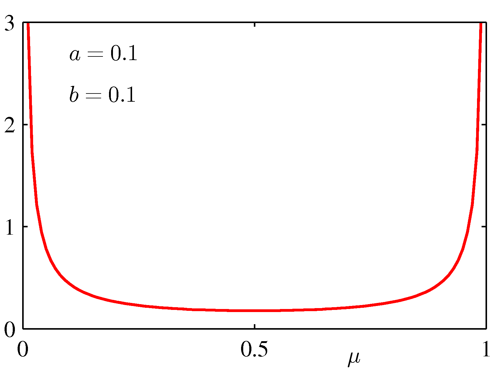
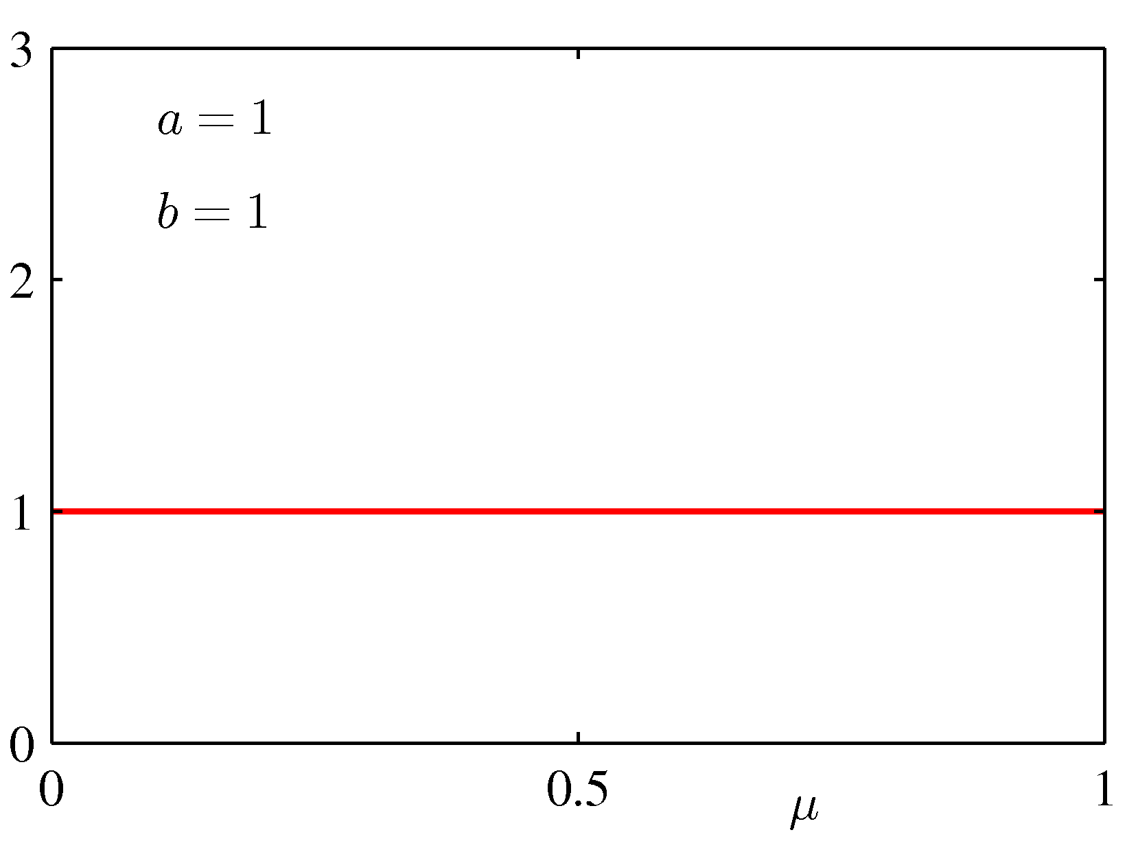
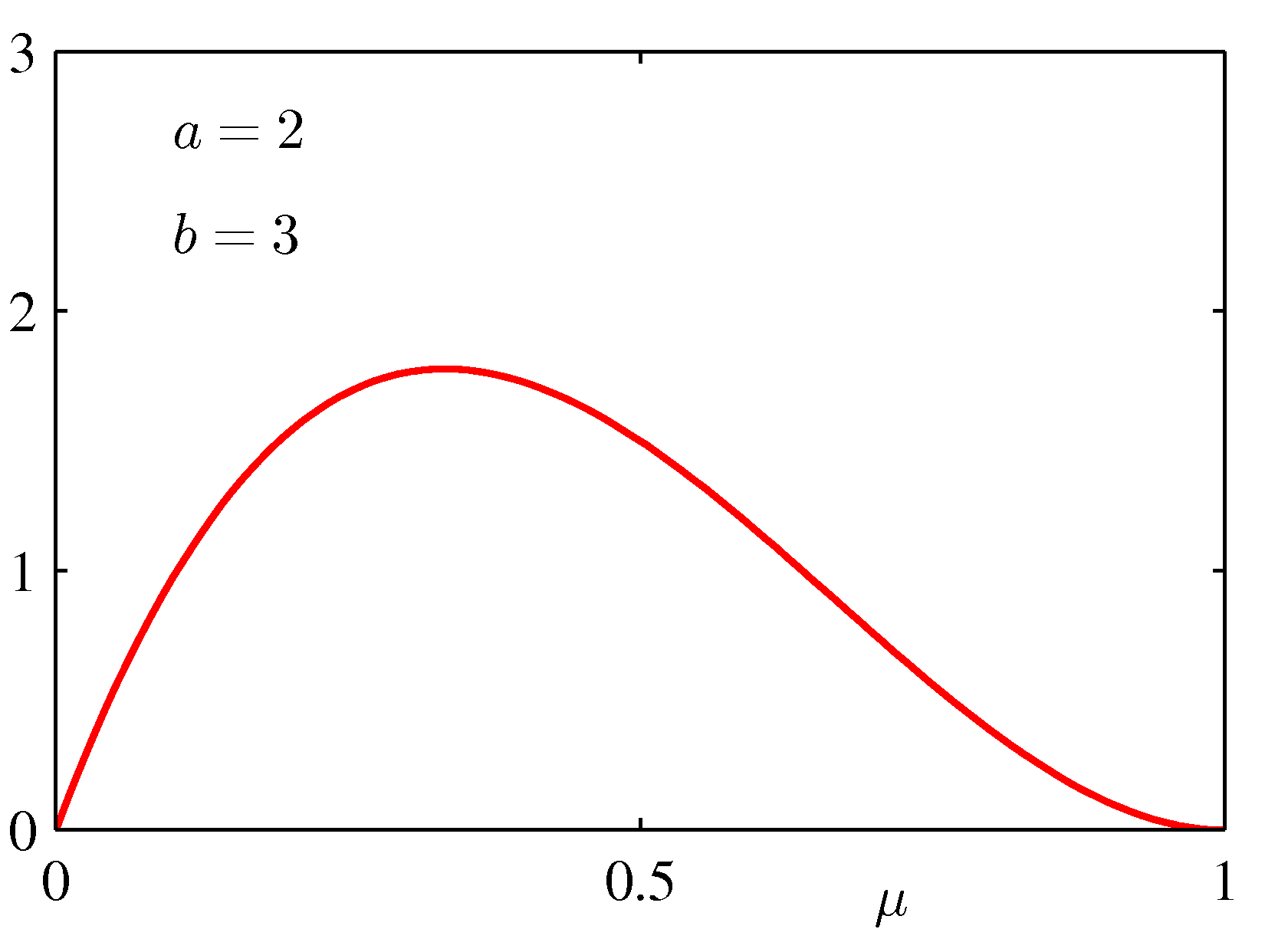
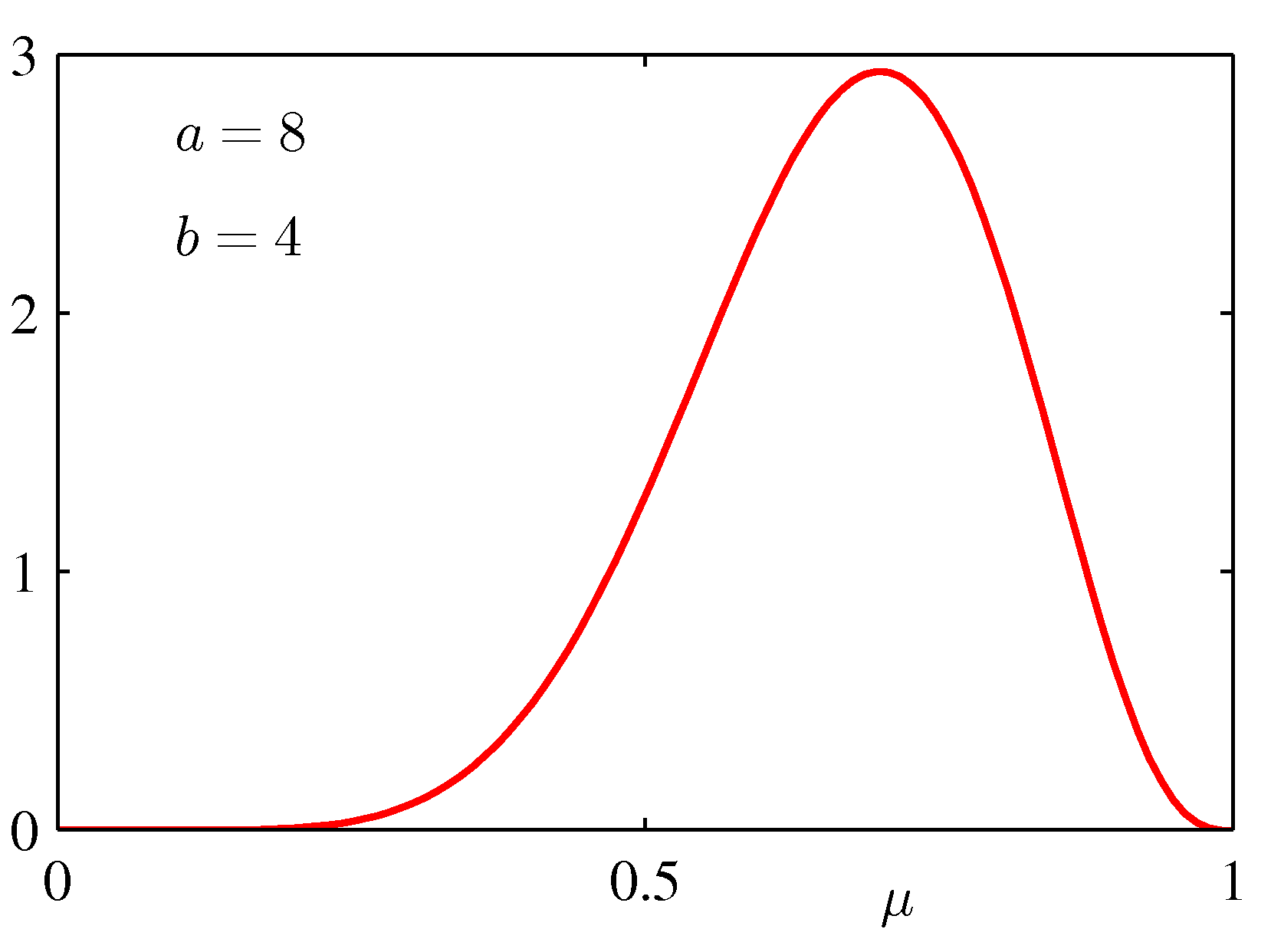
for various values of the hyper-parameters a and b is shown below:
The mean and variance of the Beta distribution are:
E[μ] = a / (a+b)
var[μ] = ab / (a+b)2(a+b+1)
If we have strong belief about a particular value μprior, we will choose a and b
such that E[μ] = μprior, and so that var[μ] is small. If we do not have
strong preferences for the prior, we will choose a and b so that Beta looks almost like a
uniform prior (a = 1 and b = 1).
Deriving the MAP Estimate of the Binomial Distribution with a Beta Prior
The MAP estimator is defined as:
μMAP = argmax μ [p(μ|D)] = argmax μ [p(D|μ)p(μ)]
μMAP = argmax μ [log p(D|μ) + log p(μ)]

Recall that:
μMLE = argmax μ [log p(D|μ)]
Hence, μMLE = μMAP only when p(μ) is a constant that does not depend on μ.
The only prior which meets this condition is the flat uniform prior for μ. MLE is the special case of MAP
for a uniform prior.
Let us now compute μMAP with a Beta prior:
p(μ) = Beta(μ | a, b) = Γ(a+b) / Γ(a)Γ(b) μa-1(1-μ)b-1
Bin(m|N,μ) = (N m) μm(1-μ)N-m
We can write the same using the ~ notation:
μ ~ Beta(a, b)
m ~ Bin(μ, N)
Under these conditions, we compute the MAP:
μMAP = argmax μ [log p(D|μ) + log p(μ)]

We compute the derivation of the terms:
l(μ) = p(D|&mu) * p(μ) = (N m) μm(1-μ)N-m * Γ(a+b) / Γ(a)Γ(b) μa-1(1-μ)b-1
l(μ) = (N m) Γ(a+b) / Γ(a)Γ(b) μm+a-1(1-μ)N-m+b-1

log l(μ) = log [(N m) Γ(a+b) / Γ(a)Γ(b)] + (m+a-1)log(μ) + (N-m+b-1)log(1-μ)

d log l(μ) / dμ = (m+a-1)/μ - (N-m+b-1)/(1-μ)
By solving d log l(μ)/dμ = 0 we obtain μMAP:
μMAP = (m + a - 1) / (N + a + b - 2)
Example:
Assume we toss a coin 3 times and obtain 3 times Tails.
In this case, D = (0,0,0).
μMLE = 0 (a very extreme conclusion -- the coin will always drop on Tails).
If we take a prior Beta(2,3) - see the bottom left graph above, which indicates a preference with a peak preference for μ = 0.4 -- then μMAP = 1/6 (a less extreme conclusion).
If we take a prior Beta(8,4) - see the bottom right graph above, which indicates a preference with a peak preference for μ = 0.6 -- then μMAP = 7/13, our peak preference is reduced, but remains quite high, because our prior was very strong, and 3 observations were not sufficient to force our conclusion more.
Bayesian Estimate of the Binomial
We now describe how to characterize the Bayesian estimation of a Binomial distribution.
In this case, we do not obtain a pointwise estimator (the "best possible μ") but instead,
we construct a new distribution that reflects our updated belief on the likely values of μ
given the dataset D.
If we choose a Beta conjugate prior for μ, we derive from Bayes theorem:
Assume:
Prior μ ~ Beta(a, b)
      X ~ Bin(μ, N)

p(μ|m,l,a,b) ∝ μm+a-1(1-μ)l+b-1

where m is the number of 1s and l = N-m is the number of 0s observed in the dataset D,
and a and b are hyper-parameters that determine our prior knowledge about p(μ).
If we observe this distribution, we realize it has the form of a Beta distribution as well (which is exactly what we wanted to achieve by choosing a conjugate prior).
The posterior of the binomial given a dataset with (m draws of 1, l=N-m draws of 0)
and a prior Beta(a,b) is: Beta(a+m, b+l)
We can interpret this using a notion of "pseudo-counts": we stated our prior knowledge about μ by saying it follows a Beta distribution with hyper-parameters a and b -- the
parameters a and b correspond intuitively to the counts of observations we "think we have seen in the past". New observations correct the a priori belief of the pseudo-counts
a and b by merging in the observed actual counts m and l. In contrast to the MLE estimator, the update of the counts is "smoothed" -- we do not jump to the conclusion that
the distribution goes according to m and l (the MLE estimate corresponds to the prior Beta(m,l)), but smoothly merge in (a,b) into (a+b, m+l).
Another way of saying this is to imagine a sequential Bayesian update process: assume that instead of updating our posterior belief for a whole dataset of N observations
at once, we update our belief sequentially, for each observation point, one by one. In this way, our prior can start from a uniform distribution (which happens to be Beta(1,1)),
and for each datapoint, we update the distribution by adding one to either the a hyper-parameter (if the datapoint is 1) or to the b hyper-parameter (if the datapoint is 0).
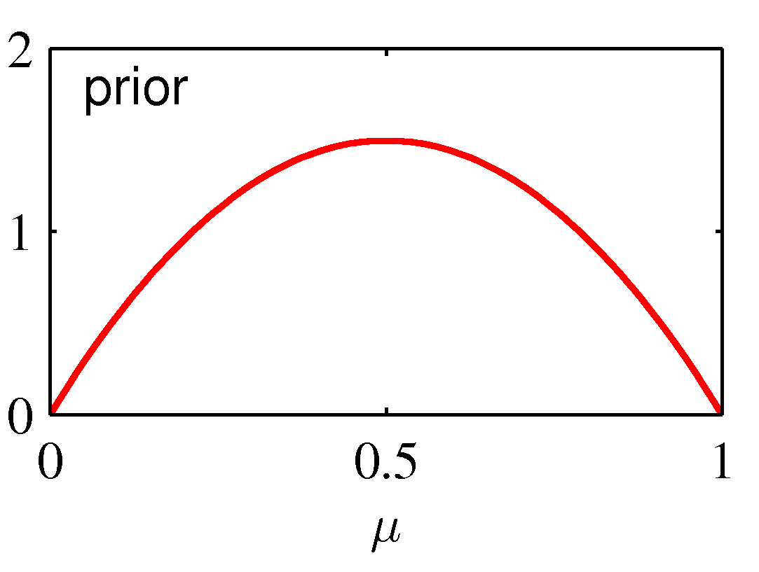
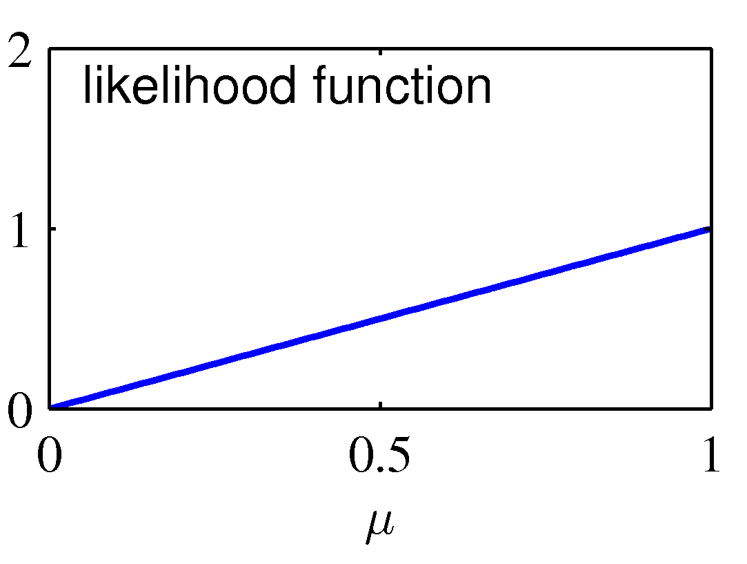
This process of sequential update is illustrated graphically below:
The graph on the left shows the prior distribution over the μ parameter: it indicates a "rough" preference for a fair Bernouilli experiment (E(μ)=0.5) with
high variance (low certainty) encoded as a Beta(2,2) prior distribution. The likelihood function is shown in the center diagram, corresponds to a single observation
of N=m=1 (in which case, the MLE estimate is μ = 1). The posterior updates the prior distribution from Beta(2,2) to Beta(3,2), which shifts smoothly from 0.5 towards
1, and has lower variance than the original Beta(2,2) -- but still does not "jump" to the extreme overfitted conclusion that μ=1.
Multinomial Distribution
Multinomial variables are the extension of the binomial from binary outcomes to n-ary outcomes. The typical example is throwing a dice with K sides, the outcome can be a number between 1 and K.
This can be represented in different ways, but one of the easiest way is to encode the outcome of the experiment as an indicator vector of K dimensions, that is a vector of K dimensions with
exactly one value equal to 1 and all others to 0
v = (0 0 ... 0 1 0 ... 0): vi = 1 and vj=0 for all j≠i for i,j ∈ (1..K)
encodes the outcome i out of the 1 to K possible outcomes.
Note that in this encoding, Σxk = 1. Note p(xk = 1) = μk. Then the distribution of x is:
p(x | μ) = ∏μkxk

where μ = (μ1, ..., μK) is the parameter of the distribution and

Σμk = 1

E(x|μ) = Σp(x|μ)x = μ
If we consider the case where we repeat the trials N times, then the distribution is known as the multinomial, and the outcome is a vector with K dimensions, m = (m1...mK)
such that Σmi = N. Then the distribution is:
Mult(m1, m2, .., mK | N, μ) = (N choose  m1 ... mK)∏μkmk
      = N! / m1! ... mK!∏μkmk
Where (N choose m1 ... mK) is the number of ways one can partition N objects into K groups of size m1 ... mK.
Consider the way we can compute the likelihood of a dataset D = (x1 ... xn) where each xi = (xi1 ... xiK) is the outcome of a trial.
Then the likelihood of the dataset D is given as follows:
likelihoodD(μ) = p(D|μ) = ∏n=1..N ∏k=1..K μkxnk = ∏k=1..K μΣxnk
Call mk = Σn=1..Nxnk.
mk corresponds to the number of times the outcome of the experiment is k -- with Σk=1..Kmk=N.
We see that the likelihood of D only depends on (mk) and not on the full details of the distribution xnk. We say in such a case that
the K numbers mk form sufficient statistics for the likelihood.
likelihoodD(μ) = p(D|μ) = ∏k=1..K μkmk

log-likelihood(μ) = Σk=1..K mk ln(μk)
The parameter of the multinomial distribution is a vector μ = (μ1, ..., μK) which is a K-dimension vector
(as opposed to a single number parameter for a binomial distribution).
For Bayesian inference, we introduce a conjugate prior on the multinomial which is a direct generalization of the Beta distribution introduced for the binomial distribution.
This conjugate distribution is called the Dirichlet distribution and is defined as:
Dirichlet(μ | α) = Γ(α0) / Γ(α1) ... Γ(αK) ∏μkαk-1

where α0 = Σαk
and   μ = (μ1,..., μK)
The Dirichlet distribution is a distribution over vectors.
Going through computation similar to the case of the binomial, we obtain the step of Bayesian inference over a multinomial distribution as follows:
p(μ | D, α) ∝ p(D | μ) p(μ | α) ∝ ∏μkαk+mk-1

and hence, exploiting the conjugacy of the Dirichlet prior:

p(μ | D, α) = Dirichlet(μ | α+m)
Each time one draws from the Dirichlet distribution, we obtain the parameters of a multinomial distribution.
The following tutorial on
Structured Bayesian Nonparametric Models with Variational Inference by Percy Liang and Dan Klein (2007) provides
excellent intuitive illustration of the Dirichlet distribution.
Last modified Nov 27th, 2012