The performance of the selected function can be measured using accuracy (how many of the predicted decisions are correct as a percentage), or for each label (Dupont / Fairfax) precision (how many labels predicted as Dupont are indeed Dupont) and Recall (how many among the Dupont apartments are labeled as Dupont by our function) and F-measure (the combination of precision and recall).
Using Scikit-Learn in Python for Classification
The Scikit-Learn library in Python provides a comprehensive and
effective platform to perform ML tasks. It implements most of the well-known ML training algorithms and provides a
well-designed API (interface) to perform the standard tasks of dataset preparation (feature extraction, feature analysis),
training and prediction, performance analysis and error analysis.
The Digits Classification
example from the Scikit-Learn tutorial illustrates the ML methodology on a prepared dataset of bitmaps of digits.
Using Numpy
Numpy is a central package in all Python machine learning libraries. It is an efficient implementation of algebraic data types
and operations.
Read the very short intro to Python and Numpy in Python Number tutorial.
Read the refresher in Python / Numpy / Matplotlib refresher
(notebook).
Interpreting the output of Models: Probability Distributions
In most classification models we will use, we will interpret the score computed by the learned function as the probability
that a sample (the feature vector encoding the object) belongs to a class. In other terms, the learned function returns
a probability distribution of size C (the number of classes) - (l1, ..., lC) such that li is in [0.0 ... 1.0] and sum(li) = 1.0. This is the basic intuition behind the algorithm called logistic regression.
One way to obtain a distribution given an arbritrary score (a floating point) is to apply a "squashing function" such as the sigmoid function:
σ(x) = 1 / 1+exp(-x)
The sigmoid maps the full range of real numbers into the interval [0,1] (it has an S-shape - hence its name).
For a binary classification case, the probability of class membership is modeled as:
prob(x ∈ class) = σ(Wx + b)
This is generalized to the case of multi-class prediction by using the softmax function, which takes as input a vector
of n-dimensions and returns a discrete distribution over n classes.
softmax([v1, ..., vn]) = [ev1 / Σk in 1..n evk, ..., evn / Σk in 1..n evk]
When multiple classes are considered, the decision function to predict one class out of C classes has the form:
y = argmaxl in [1..C] softmax(W.x + b)[l]
Preparing Datasets
Before the classifier methods of fit() and predict() can be used, the dataset must be encoded as the simple algebraic representation
we illustrated above (matrix of floating point values). This is performed by selecting feature extraction functions,
which are functions which compute one numeric value given an object to classify.
The feature extraction process can be more complex than just extracting computed features from observable objects.
It can include steps of normalization (around the average and standard deviation of the range of values for a given feature) and dimensionality reduction (algebraic transformation which projects a vector of dimension N to a vector
of dimension P such that P is much smaller than N). Such transformations must be applied according to the mathematical
expectations of the training algorithm.
In Scikit-learn, the feature_extraction
and transform modules are used to implement dataset preparation.
Feature extraction includes so called vectorizers.
Several transformers are provided in the library to perform standard data transformation tasks.
Vectorizers and transformers can be combined into efficient pipelines.
Features for NLP Applications
The Scikit-learn documentation
on text feature extraction summarizes the key features used in NLP applications.
How can we encode text - which is a sequence of discrete letters, words, sentences of arbitrary length - into the sort of fixed size vectors
and matrices expected by the ML method described above?
The key features representations we will encounter are:
- Bag of words
- Tf-idf weights
- Window-based features (current word, previous word, next word in sentence)
- Parts-of-speech features
The basis of these representations are:
- Encodings of basic linguistic units
- Combination of these encodings
For example, to represent the occurrence of a word wi in a document, we can use a vector of size W = | Vocabulary |
(in general - W is about 200,000) which has one element for each possible word in the vocabulary. The vector representation
of word wi is thus the vector (0,0...,0,1,0...,0) with all values equal to zero except that at index i.
This encoding is called the one-hot encoding of the vocabulary.
Given this representation, we can combine the information that multiple words are present in a document by just summing up the vectors
representing each word. Thus a document (w1 ... wD) is encoded a Σi in [1..D] vwi.
This method is called the Bag of Words (BoW) encoding of the document.
Note that this BoW representation loses the information of the order in which words occur in the document - so that "Avi stole from Betty" and
"Betty stole from Avi" are represented by the same vector.
The BoW representation can be made more effective for certain tasks by taking into account the frequency of the words within the document - so that more frequent words are given higher weight than less frequent ones.
Another variant of BoW considers the relative frequency of words within the given document as opposed to all the other documents in a dataset.
This method is called the TF*IDF weighting scheme.
Another weakness of the BoW encoding is that it does not take into account the relative similarity of word meanings. For example,
the two sentences "John hit Bob" and "John hurt Bob" are encoded into two vectors that are as distant from each other as the vector
encoding of "John likes Bob". In many tasks, we want to take advantage of the fact that some words are more similar to each other than others
(reflecting lexical relations such as synonymy). The BoW representation cannot achieve this, since all word representations are orthogonal
to each other - and thus distant to each other in the same manner.
From Feature-based Supervised ML to Deep Learning
One can think of the transition from the traditional ML method to the Deep Learning method in multiple ways.
One of them is to put the focus on learning representation - that is, the DL method attempts to include
within the scope of the learning optimization the task of encoding the input features in an effective manner.
Another perspective is to define the ML approach as a way to combine multiple representations, at different levels of abstraction,
in an effective manner.
The last aspect of the method is the focus on a specific family of functions to drive the learning process which is more general
than the linear / log-linear family we have used as an example so far.
Learning as Function Optimization - Loss Functions and Regularization
Let us first re-state the task of training a ML model as a task of optimizing a function.
The goal of training is, given a dataset (x,y), to characterize a function f() such that the predictions ŷ = f(x)
over the training dataset are as accurate as possible. The function f() is characterized by a set of parameters θ
and belongs to a pre-set family of functions (for example, linear functions, log-linear functions).
To formalize the notion of "a function that is accurate over a dataset", we introduce the concept of loss function.
The loss function determines how far a prediction is from the expected result on a given sample. L(ŷ, y) measures
how the distance between a predicted value and the real value y. The loss function should be bounded on the minimum, so that,
in general, L(ŷ, y) = 0 only when ŷ = y.
The optimization task we consider is thus:
Find θ such that the loss over all the training dataset is minimized.

θ* = argminθ 1/n Σ(x,y) ∈ Dataset L(fθ(x), y)
Loss Functions
Loss Functions that are often used include:
- For regression problems (y is a scalar value), we use either:
L1(ŷ, y) = |ŷ - y|
or L2 = (ŷ - y)2
- For binary classification problems: the predicted output is either -1 or +1 and the decision rule is that ŷ has the same sign as y.
The loss function is
Lhinge = max(0, 1-ŷy)
- Binary cross-entropy (logistic loss): the predicted output models p(y=1|x), and the decision rule is ŷ > 0.5 for a positive classification. The binary cross-entropy loss is:
Lbce(ŷ,y) = -ylog(ŷ) - (1-y)log(1-ŷ)
- Cross-entropy loss (negative log-likelihood): the predicted output models ŷ = (ŷ1 ... ŷC) is
a distribution over the C possible classes. ŷ is in general the output of a softmax function applied to scores in C dimension.
Lnll(ŷ,y) = -Σi ∈ (1..C) yilog(ŷi).
When y is a deterministic distribution (a one-hot distribution) when t ∈ (1..C) is the correct class, we obtain:
Lnll(ŷ,y) = -log(ŷt)
Regularization
When we optimize for the loss functions listed above, there is a risk to obtain a solution θ* which overfits the
training dataset. This is particularly the case when the family of functions over which we search a solution is expressive.
To avoid overfitting, we introduce a term called regularization which imposes desirable constraints on the form of the solution.
Usually, the regularization term measures the complexity of the returned function. We prefer in general simple solutions
(which are deemed to be more general) than complex ones.
We search for a solution which combines low loss and low regularization:
θ* = argminθ (1/n Σi = 1..n L(f(xi, θ), yi) + λ R(θ))
It is common to use the L2 measure of complexity for the regularization term R(θ) = L2(θ).
Gradient Descent Algorithm
There are different ways to solve the optimization problem above algorithmically. One effective and very general method
is the algorithm of stochastic gradient descent (taken here from the formulation in [Goldberg 2017, 2.8.1]):
Algorithm: Online Stochastic Gradient Descent Training
Input:
- Function f(x; θ) parameterized with parameters θ
- Training set of inputs x1 ... xn and desired outputs y1 ... yn
- Loss function L
while stopping criteria not met do
Sample a training example xi; yi
Compute the loss L(f(xi; θ); yi)
ĝ ← gradients of L(f(xi; θ); yi) w.r.t θ
θ ← θ - ηt ĝ
return θ
For well-chosen loss functions and families of functions f(), the computation of the gradients can be made efficient and automated.
Representation - Learning Feature Mapping
The XOR Problem
The XOR problem is a well-known case of a non-linearly separable function:
We want to learn a mapping from 2 boolean variables (x1, x2) to the function xor(x1, x2).
But there is no solution to the optimization problem:
W ∈ ℜ2, b ∈ ℜ
- W . (0; 0) + b < 0
- W . (0; 1) + b >= 0
- W . (1; 0) + b >= 0
- W . (1; 1) + b < 0
However, if we feed the input x into a non-linear function φ, we can find a solution to this optimization problem.
For example, consider:
φ(x1, x2) = (x1x2, x1+x2)

ŷ = f(x) = W . φ(x) + b
Feed-Forward Neural Networks as Universal Approximators
The question we must now solve becomes how to find a good function φ to make our problem separable.
This has been addressed in the ML field with so-called Kernel methods - where general functions φ turn an input problem x of
dimension n into a problem with much higher dimension N.
The deep learning approach is different and consists of learning a trainable non-linear mapping function φ of a specific form.
The general form of this trainable mapping we consider is:
ŷ = W φ(x) + b
φ(x) = g(W'x + b')

where g is a non-linear function
This formulation corresponds to the simplest neural-network architecture, called the Multi-layer perceptron (MLP).
In general, we can combine multiple layers of this form, where a composition of linear mapping from din to dout
is followed by a non-linear function g(). This leads to the general definition of an architecture called feed-forward neural network (FFNN).
The architecture of such functions is described as a sequence of equations of the form:
NNMLP2(x) = y
    h1 = g1(W1 x + b1)
    h2 = g2(W2 h1 + b2)
    y = W3 h2
It was proven in Cybenko, Approximation by superpositions of a sigmoidal function, Mathematics of Control, Signals and Systems, 2(4), 1989 that the MLP1 architecture is a universal approximator - that is, it can approximate with any desired non-zero error functions that include all continuous functions on a closed and bounded subset of ℜn.
This result proves that an MLP solution exists for any given function to approximate, but it does not provide a constructive algorithm to find it.
In recent years, it was proven that for large classes of problems, algorithms find better solutions faster when more complex architectures (deeper layers) are used coupled with stochastic gradient descent optimization.
Non-linear layers
The non-linear functions used typically in deep-learning include the following:
- Sigmoid: σ(x) = 1/1+e-x maps x to the range [0,1] (it has a S-shape)
- tanh: tanh(x) = (e2x-1) / (e2x+1) maps x to the range [-1,1]
- Relu: (rectifier linear unit) ReLU(x) = max(0,x)
Neural Language Models
Let us return to the task of learning a language model using the deep learning methodology.
The task we consider is to predict what is the next word given the sequence of preceding words in a document.
Formally, we want to learn the conditional distribution:
p(wi+1 | w1:i)
We learned count-based method in the previous lecture - and found a solution to this task by using n-gram models.
The limitations of n-gram models are:
- They require extremely large memory (exponential in the size of the history we consider - |V|n where n is the size of the n-gram and |V| is the size of the vocabulary.
- Consequently, they have limited memory to deal with long-range dependencies (cases where the next token depends on the token that appeared 15 positions in the past)
- They suffer from lack of generalization: if an n-gram was never observed at training time, it is complex to predict its likelihood. Complex smoothing methods limit this problem but do not solve it completely.
Neural Language Models (NLMs) were introduced to address these limitations. The key advantage of NLMs is that they can handle long histories with a small (linear) increase in the number of parameters in the model. The first influential description of this approach is in
A Neural Probabilistic Language Model, Y. Bengio et al, 2003.
The input of this model is an n-gram w1:k and the output is a probability distribution over the vocabulary V.
The words in the n-gram are first mapped to one-hot vectors of size V.
These vectors are then mapped to encoding vectors of size dw.
The input vector is the concatenation of these embedding vectors -
x = [v(w1); ...; v(wk)].
The vector x is then pushed to an MLP with one hidden layer:
y = p(wi | w1:k) = LM(w1:k) = softmax(W2h + b2)
h = g(W1x + b1)
Counting the number of parameters in this model, we obtain:
wi ∈ ℜ|V| (|V| ~ 10,000 - one-hot encoding)
v(wi) ∈ ℜdw
v(wi) = E.w - E ∈ ℜ|V| x dw
W1 ∈ ℜk x dw x dh
b1 ∈ ℜdh
W2 ∈ ℜdh x |V|
b2 ∈ ℜ|V|
To train this model, we iterate over a corpus of text, and feed as training pairs every observed pair of (n-gram of k words, wk+1).
For a corpus of size C tokens, we obtain about C such pairs.
The loss function we use is cross-entropy - which compares the predicted distribution over |V| words with the observed word wk+1.
The space efficiency of this method is much better than n-gram based LMs, but the training time and prediction time is much higher - mainly because
of the cost of the softmax function over vectors of size |V|.
Last modified 28 Oct 2018
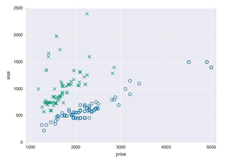 The task we address is that of predicting which of two neighborhoods an apartment is located
at, based on the apartment's price and size. The diagram shows a plot of some apartments,
where the x-axis denotes the monthly rent price in USD, while the y-axis is the size in
square feet. The blue circles are for Dupont Circle, Washington DC and the green crosses are in Fairfax, VA.
We observe that the data points corresponding to the two classes can be separated by a line going across the plane (x,y).
This is called a linearly-separable dataset. It is the easiest case for machine learning.
The encoding of this classification task as an ML task adopts the following steps:
The task we address is that of predicting which of two neighborhoods an apartment is located
at, based on the apartment's price and size. The diagram shows a plot of some apartments,
where the x-axis denotes the monthly rent price in USD, while the y-axis is the size in
square feet. The blue circles are for Dupont Circle, Washington DC and the green crosses are in Fairfax, VA.
We observe that the data points corresponding to the two classes can be separated by a line going across the plane (x,y).
This is called a linearly-separable dataset. It is the easiest case for machine learning.
The encoding of this classification task as an ML task adopts the following steps: