This assignment covers 2 parts:
Make sure you have installed scipy, scikit-learn and numpy to work on this assignment. This should be already available if you have installed the Anaconda distribution.
Submit your solution in the form of a Jupyter notebook file (with extension ipynb). The notebook should be readable - use the capability of notebooks to use markup language for well formatted text with headings / bold / italics as needed. The notebook should tell a story - what is it you are testing, what do you expect to see, what do you observe after running an experiment. Images should be submitted as PNG or JPG files. The whole code should also be submitted as a separate folder with all necessary code to run the questions separated in clearly documented functions.
Look at the following two notebooks as examples to get you started - copy them to your Anaconda folder, then start your Jupyter notebook server and explore them:
Lookup at the data of the Brown corpus as it is stored in the nltk_data folder (by default, it is in a folder named like C:\nltk_data\corpora\brown under Windows). The format of the corpus is quite simple. We will attempt to add a new "section" to this corpus.
A dataset used in many articles studying language models is the Penn Tree Bank (PTB) dataset, which contains 929k training words, 73k validation words, and 82k test words. It has the 10k most frequent words in its vocabulary. Tomas Mikolov’s webpage distributes a version of this dataset which has been pre-processed such that only the top-10K most frequent words occur, the others are replaced by the token <unk>, words are separated with spaces according to consistent tokenization rules, numbers are replaced by a single token N, and sentences are segmented one per line. (The file takes 33MB.)
For example:
consumers may want to move their telephones a little closer to the tv set
<unk> <unk> watching abc 's monday night football can now vote during <unk> for the greatest play in N years
from among four or five <unk> <unk>
The dataset is also available in a form that is easy to process when building character-level language models (where the objective is to predict the next char, not the next word, given a history of the previous characters):
c o n s u m e r s _ m a y _ w a n t _ t o _ m o v e _ t h e i r _ t e l e p h o n e s _ a _ l i t t l e _ c l o s e r _
t o _ t h e _ t v _ s e t
< u n k > _ < u n k > _ w a t c h i n g _ a b c _ ' s _ m o n d a y _ n i g h t _ f o o t b a l l _ c a n _ n o w _
v o t e _ d u r i n g _ < u n k > _ f o r _ t h e _ g r e a t e s t _ p l a y _ i n _ N _ y e a r s _ f r o m _
a m o n g _ f o u r _ o r _ f i v e _ < u n k > _ < u n k >
These types of low-level text encoding are critical to any process of NLP.
Your task is to take as input the URL to an arbitrary text file and to format it in a way that applies the same conventions as the word-level Penn Treebank representation of Mikolov:
To identify the top-10K most frequent words, you can use the Python collections.Counter() object and its method most_common(n). You must submit:
# you need matplotlib version 1.4 or above
import matplotlib.pyplot as plt
import matplotlib
print(matplotlib.__version__)
%matplotlib inline

plt.loglog([val for word,val in corpus_counts.most_common(4000)])
plt.xlabel('rank')
plt.ylabel('frequency');
You can base your implementation either on the model described in this article (which needs to be adapted from characters to words) or in the nltk module nltk.model.ngram. (NOTE: This code is not available in nltk's codebase, but you can adjust it to your answer based on this link.) Here is Yoav Goldberg's code adapted to nltk classes and to Python3 (thanks to Ben Eyal):
def create_lm(fname, order=4):
    with open(fname) as f:
        data = f.read()
    pad = '*' * order
    data = pad + data
    cfd = nltk.ConditionalFreqDist((data[i : i + order], data[i + order]) for i in range(len(data) - order))
    cpd = nltk.ConditionalProbDist(cfd, nltk.MLEProbDist)
    return cpd

order = 4
lm = create_lm('data/shakespeare.txt', order)
out = []
hist = '*' * order
for _ in range(1000):
    letter = lm[hist].generate()
    hist = hist[1:] + letter
    out.append(letter)
print(''.join(out))
1.3.1.2 One way to improve the model is to use a smoothing technique to increase the generalization of the trained model. Learn how the nltk probability distribution module provides different estimators that implement different smoothing methods (Laplace, Lidstone, Witten-Bell, Good-Turing). Change your model to use a different estimator than the Maximum Likelihood Estimator (MLE) count-based estimator to compute the probability of p(w|history). Compare the obtained perplexity of the trained model on the development dataset for different estimators Lidstone for a variety of hyper-parameter gamma (0 < gamma < 1). Draw a graph of the obtained perplexity (or cross-entropy) on the dev test for different values of gamma.
1.3.1.3 Another way to improve the model is to use an n-gram model with increasing values of n (2,3,...10). Draw a graph of the obtained perplexity (or cross-entropy) on the dev test for different values of n between 2 and 20.
1.3.1.4 Based on the 2 graphs above, prepare the best predicted n-gram model based on a Lidstone model with an optimized gamma parameter and of the best possible n order. Test this model on the test dataset of the Penn Treebank and report results. Compare your result with the expected results on a uniform distribution of words (worst case) and on recent research results reported in research paper on language models that you can find in Google Scholar tested on the Penn Treebank dataset.
1.3.2.1 Implement the method generate(model, seed) and test it on the best model you have trained. Discuss ways to generate when the seed is shorter than the history length of the n-gram model. Discuss ways to decide when the generation should stop. In this question, when you sample from the LM given a history, pick the most likely word generated by the LM. Report at least 5 randomly generated segments on different seeds and comment on what you observe.
1.3.2.2 In the method above, we always generate the next token based on the previous history by picking the most likely candidate predicted by the LM. For a given seed, this method will generate deterministic output. The way to generate more variety given a probabilistic model is to introduce a parameter usually called the temperature of the generator which allows us to sample words randomly according to the distribution produced by the LM (that is, we do not always select the most likely candidate - we sample from the distribution produced by the LM).
Read Maximum Likelihood Decoding with RNNs - the good, the bad, and the ugly by Russell Stewart (2016) and explain how a temperature argument can control the level of variability generated by the model.
Read the code in generator.py from Sameer Sing which demonstrates a method to generate from a LM with a temperature parameter. Explain how the code in this method corresponds to the mathematical explanation provided in the blog above.Read the following article: The Unreasonable Effectiveness of Recurrent Neural Networks, May 21, 2015, Andrej Karpathy (up to Section "Further Reading"). Write a summary of this essay of about 200 words highlighting what is most surprising in the experimental results reported in the blog.
Read the follow-up article: The unreasonable effectiveness of Character-level Language Models (and why RNNs are still cool), Sept 2015, Yoav Goldberg. Write a summary of this essay of about 200 words.
Strikingly realistic output can be generated when training a character language-model on a strongly-constrained genre of text like cooking recipes. Train Yoav Goldberg's n-gram model on the dataset provided in do androids dream of cooking? which contains about 32K recipes gathered from the Internet.
Your task is:
In this question, we will reproduce the polynomial curve fitting example used in Bishop's book in Chapter 1. Polynomial curve fitting is an example of a learning task called regression (as opposed to classification we discussed in class). In regression, the objective is to learn a function mapping an input variable X to a continuous target variable Y, while in classification, Y is a discrete variable. For educational purposes, it turns out that regression is simpler to grasp than classification. This task shows how to develop a probabilistic model of a task often described in geometric terms.
The outline of the task is:
Generate a dataset of points in the form of 2 vectors x and t of size N where:
ti = y(xi) + Normal(mu, sigma)

where the xi values are equi-distant on the [0,1] segment (that is, x1 = 0, x2=1/N-1, x3=2/N-1..., xN = 1.0)
mu = 0.0
sigma = 0.03
y(x) = sin(2πx)
Our objective will be to "learn" the function y from the noisy sparse dataset we generate.
The function generateDataset(N, f, sigma) should return a tuple with the 2 vectors x and t. N is the number of samples to generate, f is a function, and sigma is the standard deviation for the noise.
Draw the plot (scatterplot) of (x,t) using matplotlib for N=100. Look at the documentation of the numpy.random.normal function in Numpy for an example of usage. Look at the definition of the function numpy.linspace to generate your dataset.
Note: a useful property of Numpy arrays is that you can apply a function to a Numpy array as follows:
import math
import numpy as np
def s(x): return x**2
def f(x): return math.sin(2 * math.pi * x)
vf = np.vectorize(f)        # Create a vectorized version of f

z = np.array([1,2,3,4])

sz = s(z)                   # You can apply simple functions to an array
sz.shape                    # Same dimension as z (4)

fz = vf(z)                  # For more complex ones, you must use the vectorized version of f
fz.shape
y(x) = w0 + w1x + w2x2 + ... + wMxMOur objective is to estimate the vector w = (w0...wM) from the dataset (x, t).
We first attempt to solve this regression task by optimizing the square error function (this method is called least squares:
Define: E(w) = 1/2Σi(y(xi) - ti)2
             = 1/2Σi(Σkwkxik - ti)2
If t = (t1, ..., tN), then define the design matrix to be the matrix Φ such that Φnm = xnm = Φm(xn).
We want to minimize the error function, and, therefore, look for a solution to the linear system of equations:
dE/dwk = 0 for k = 0..MWhen we work out the partial derivations, we find that the solution to the following system gives us the optimal value wLS given (x, t):
wLS = (ΦTΦ)-1ΦTt

(Note: Φ is a matrix of dimension Nx(M+1), w is a vector of dimension (M+1) and t is a vector of dimension N.)
Here is how you write this type of matrix operations in Python using the Numpy library:
import numpy as np
import scipy.linalg

t = np.array([1,2,3,4])                    # This is a vector of dim 4
t.shape                                    # (4,)
phi = np.array([[1,1],[2,4],[3,3],[2,4]])  # This is a 4x2 matrix
phi.shape                                  # (4, 2)
prod = np.dot(phi.T, phi)                  # prod is a 2x2 matrix
prod.shape                                 # (2, 2)
i = np.linalg.inv(prod)                    # i is a 2x2 matrix
i.shape                                    # (2, 2)
m = np.dot(i, phi.T)                       # m is a 2x4 matrix
m.shape                                    # (2, 4)
w = np.dot(m, t)                           # w is a vector of dim 2
w.shape                                    # (2,)
Implement a method OptimizeLS(x, t, M) which given the dataset (x, t) returns the optimal polynomial of degree M that approximates the dataset according to the least squares objective. Plot the learned polynomial w*M(xi) and the real function sin(2πx) for a dataset of size N=10 and M=1,3,5,10.
We define a new objective function:
Define EPLS(w) = E(w) + λEW(w)

Where EPLS is called the penalized least-squares function of w
and   EW is the penalty function.

We will use a standard penalty function:
      EW(w) = 1/2 wT.w = 1/2 Σm=0..Mwm2
When we work out the partial derivatives of the minimization problem, we find in closed form, that the solution to the
penalized least-squares is:
wPLS = (ΦTΦ + λI)-1ΦTtλ is called a hyper-parameter (that is, a parameter which influences the value of the model's parameters w). Its role is to balance the influence of how well the function fits the dataset (as in the least-squares model) and how smooth it is.
Write a function optimizePLS(x, t, M, lambda) which returns the optimal parameters wPLS given M and lambda.
We want to optimize the value of λ. The way to optimize is to use a development set in addition to our training set.
To construct a development set, we will extend our synthetic dataset construction function to return 3 samples: one for training, one for development and one for testing. Write a function generateDataset3(N, f, sigma) which returns 3 pairs of vectors of size N each, (xtest, ttest), (xvalidate, tvalidate) and (xtrain, ttrain). The target values are generated as above with Gaussian noise N(0, sigma).
Look at the documentation of the function numpy.random.shuffle() as a way to generate 3 subsets of size N from the list of points generated by linspace.
Given the synthetic dataset, optimize for the value of λ by varying the value of log(λ) from -40 to -20 on the development set. Draw the plot of the normalized error of the model for the training, development and test for the case of N = 10 and the case of N=100. The normalized error of the model is defined as:
NEw(x, t) = 1/N [Σi=1..N[ti - Σm=0..Mwmxim]2]1/2Write the function optimizePLS2(xt, tt, xv, tv, M) which selects the best value λ given a dataset for training (xt, tt) and a development test (xv, tv). Describe your conclusion from this plot.
tn = y(xn; w) + εnWe now model the distribution of εn as a probabilistic model:
εn ~ N(0, σ2)

since tn = y(xn; w) + εn:

p(tn | xn, w, σ2) = N(y(xn; w), σ2)
We now assume that the observed data points in the dataset are all drawn in an independent manner (iid), we can then express the likelihood of the whole dataset:
p(t | x,w,σ2) = ∏n=1..Np(tn | xn, w, σ2)
              = ∏n=1..N(2πσ2)-1/2exp[-{tn - y(xn, w)}2 / 2σ2]
We consider this likelihood as a function of the parameters (w and σ) given a dataset (t, x).
If we consider the log-likelihood (which is easier to optimize because we have to derive a sum instead of a product), we get:
-log p(t | w, σ2) = N/2 log(2πσ2) + 1/2σ2Σn=1..N{tn - y(xn;w)}2
We see that optimizing the log-likelihood of the dataset is equivalent
to minimizing the error function of the least-squares method. That is
to say, the least-squares method is understood as the maximum
likelihood estimator (MLE) of the probabilistic model we just developed, which produces the values wML = wLS.
We can also optimize this model with respect to the second parameter σ2 which, when we work out the derivation and the solution of the equation, yields:
σ2ML = 1/N Σn=1..N{y(xn, wML) - tn}2
Given wML and σ2ML, we can now compute the plugin posterior predictive distribution, which gives us the probability distribution
of the values of t given an input variable x:
p(t | x, wML, σ2ML) = N(t | y(x,wML), σ2ML)This is a richer model than the least-squares model studied above, because it not only estimates the most-likely value t given x, but also the precision of this prediction given the dataset. This precision can be used to construct a confidence interval around t.
We further extend the probabilistic model by considering a Bayesian approach to the estimation of this probabilistic model instead of the maximum likelihood estimator (which is known to over-fit the dataset). We choose a prior over the possible values of w which we will, for convenience reasons, select to be of a normal form (this is a conjugate prior as explained in our review of basic probabilities):
p(w | α) = ∏m=0..M(α / 2π)1/2 exp{-α/2 wm2}
             = N(w | 0, 1/αI)
This prior distribution expresses our degree of belief over the values that w can take.
In this distribution, α plays the role of a hyper-parameter (similar to λ in the regularization model above).
The Bayesian approach consists of applying Bayes rule to the estimation task of the posterior distribution given the dataset:
p(w | t, α, σ2) = likelihood . prior / normalizing-factor
                = p(t | w, σ2)p(w | α) / p(t | α, σ2)
Since we wisely chose a conjugate prior for our distribution over w, we can compute the posterior analytically:
p(w | x, t, α, σ2) = N(μ, Σ)

where Φ is the design matrix as above:

μ = (ΦTΦ + σ2αI)-1ΦTt

Σ = σ2(ΦTΦ + σ2αI)-1
Given this approach, instead of learning a single point estimate of w as in the least-squares and penalized least-squares methods above, we have inferred a distribution over all possible values of w given the dataset. In other words, we have updated our belief about w from the prior (which does not include any information about the dataset) using new information derived from the observed dataset.
We can determine w by maximizing the posterior distribution over w given the dataset and the prior belief. This approach is called the maximum posterior (usually written MAP). If we solve the MAP given our selection of the normal conjugate prior, we obtain that the posterior reaches its maximum on the minimum of the following function of w:
1/2σ2Σn=1..N{y(xn, w) - tn}2 + α/2wTw
We find thus that wMAP is in fact the same as the solution of the penalized least-squares method for λ = α σ2.
In other words - this probabilistic model explains that the PLS is in fact the optimal solution to the problem when our prior belief on the parameters w is
a Normal distribution N(0, 1/αI) which encourages small values for the parameter w.
A fully Bayesian approach, however, does not look for point-estimators of parameters like w. Instead, we are interested in the predictive distribution p(t | x, x, t). The Bayesian approach consists of marginalizing the predictive distribution over all possible values of the parameters:
p(t | x, x, t) = ∫ p(t|x, w)p(w | x, t) dw(For simplicity, we have hidden the dependency on the hyper-parameters α and σ in this formula.) On this simple case, with a simple normal distribution and normal prior over w, we can solve this integral analytically, and we obtain:
p(t | x, x, t) = N(t | m(x), s2(x))

where the mean and variance are:

m(x) = 1/σ2 Φ(x)TS Σn=1..NΦ(xn)tn

s2(x) = σ2 + Φ(x)TSΦ(x)

S-1 = αI + 1/σ2 Σn=1..NΦ(xn)Φ(xn)T

Φ(x) = (Φ0(x) ... ΦM(x))T = (1 x x2 ... xM)T
Note that the mean and the variance of this predictive distribution depend on x.
Your task: write a function bayesianEstimator(x, t, M, alpha, sigma2) which given the dataset (x, t) of size N, and the parameters M, alpha, and sigma2 (the variance), returns a tuple of 2 functions (m(x) var(x)) which are the mean and variance of the predictive distribution inferred from the dataset, based on the parameters and the normal prior over w. As you can see, in the Bayesian approach, we do not learn an optimal value for the parameter w, but instead, marginalize out this parameter and directly learn the predictive distribution.
Note that in Python, a function can return a function (a closure, like in Scheme or in JavaScript) using the following syntax:
def adder(x):
    return lambda(y): x+y

a2 = adder(2)

print(a2(3))       // prints 5
print(adder(4)(3)) // prints 7
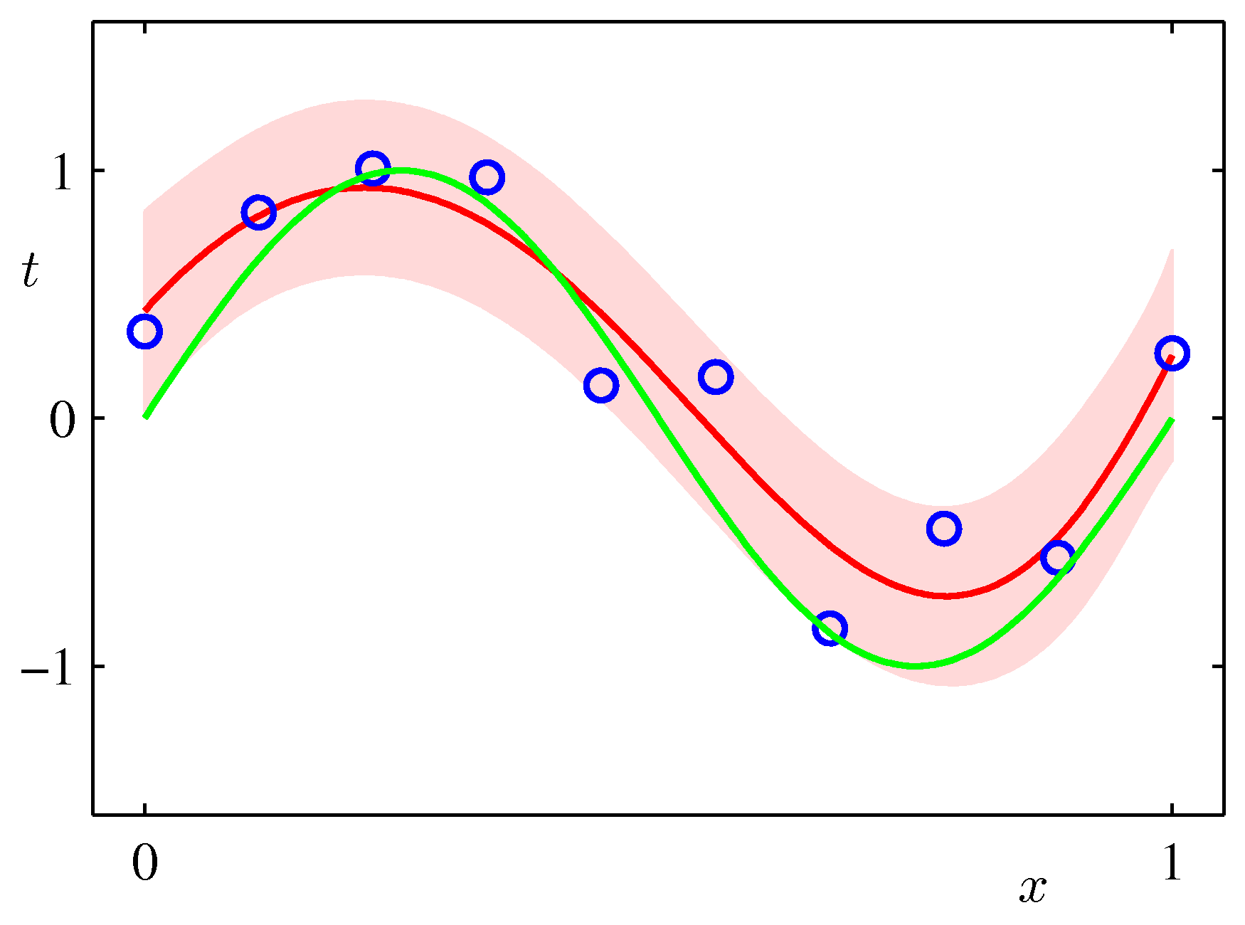
Draw the plot of the original function y = sin(2πx) over the range [0..1], the mean of the predictive distribution m(x) and the confidence interval
(m(x) - var(x)1/2) and (m(x) + var(x)1/2) (that is, one standard deviation around each predicted point) for the values:
alpha = 0.005
sigma2 = 1/11.1
M = 9
over a synthetic dataset of size N=10 and N=100. The plot should look similar to the Figure below (from Bishop p.32).
Interpret the height of the band around the most likely function in terms of the distribution of the xs in your synthetic dataset. Can you think of ways to make this height very small in one segment of the function and large in another?