Bayesian Concept Learning
Reference: Machine Learning - a Probabilistic Approach, Kevin Murphy 2012, Chapter 3.
Consider the task of learning a concept in the following sense:
a learner is shown a sequence of instances (objects) labeled as belonging to a concept.
For example, a child is shown an animal and is told it is a "dog" or a "cat".
Objects can belong to multiple concepts. We expect the learner to be able to generalize
on the basis of the perceived description of the instances so that unseen instances can be
categorized into the set of concepts.
We model this task as that of learning a function f(instance) mapping instances to boolean values -
f(x) = 1 indicates that x belongs to the concept represented by f, f(x) = 0 indicates x does not
belong to the concept.
The following example of this task of concept learning is called the "number game" - it was
introduced by Tenenbaum in 1999 in his PhD thesis. In this game, instances are a finite set
of integer numbers (for example, {1,2,...,100}). Concepts are described by natural language
expressions - for example "prime numbers" or "even numbers" or "powers of 2". They denote each
a subset of the instances. For example, "even numbers" denotes the subset {2,4,6...,98,100}.
The process of concept learning is modeled as incremental Bayesian model update.
The scenario of learning is illustrated by this exemple:
I want to teach you a "concept" which is a set of numbers between 1 and 100.
I tell you "16" is positive example of the concept.
What other numbers do you think are positive?
Is "17"? "6"? "32"? "99"?
Naturally, with only one example it is difficult to answer - so predictions will be vague.
When deciding on prediction, we will prefer numbers that are "similar" to "16" - but similar in what sense?
"17" is similar because it is "close" to "16", "6" is similar because it has a digit in common with "16",
"32" because it is also even and also a power of "2", "99" does not seem similar for any "good reason".
Thus some numbers are more likely than others and we can represent our predictions as a probability distribution
p(x|D) - where x is the number on which we need to make a prediction ("32" or "99") and D is the dataset we have
observed so far - initially only {"16"}. This is called the posterior predictive distribution.
We can observe this posterior predictive distribution by asking a group of people their prediction on all numbers
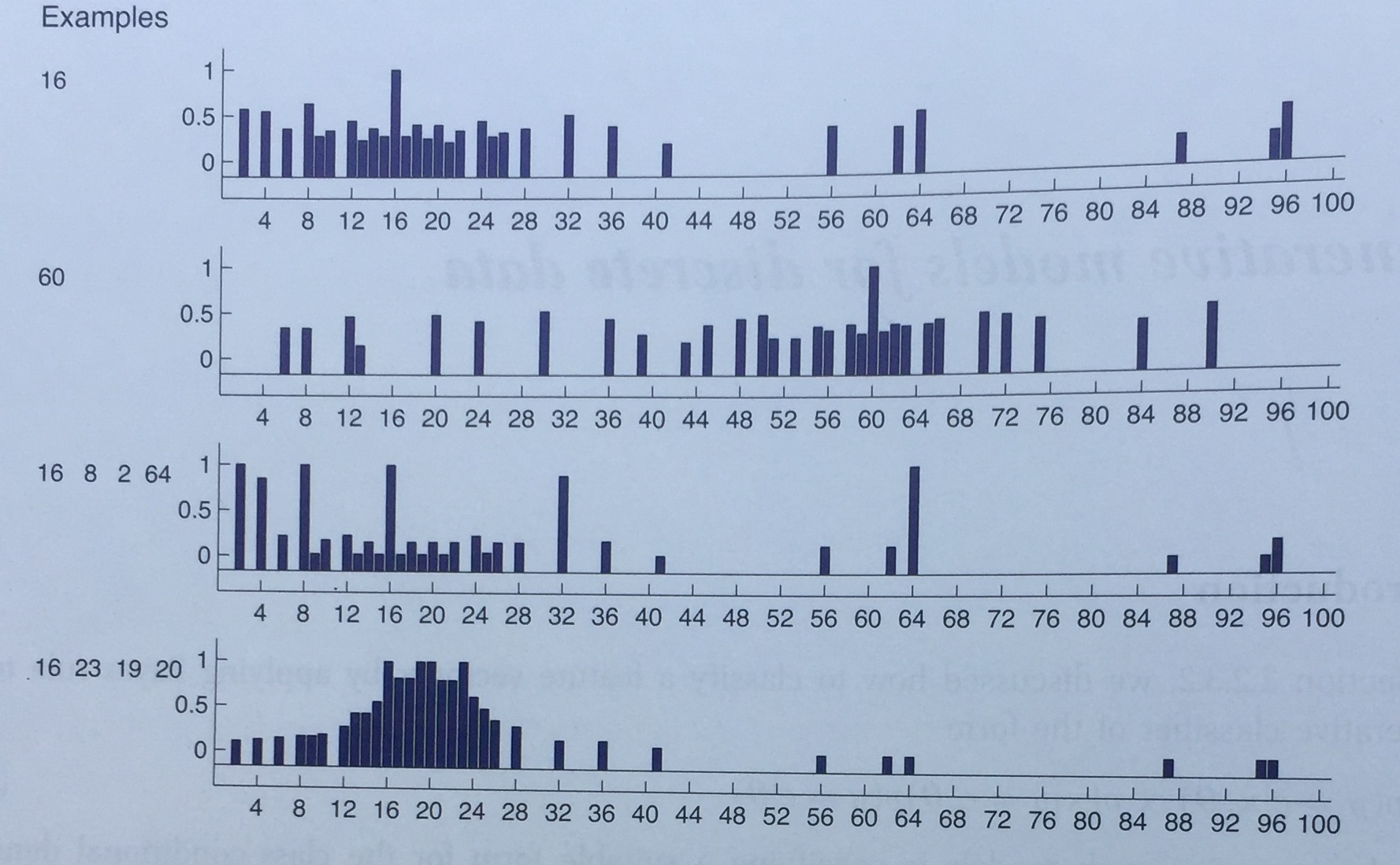
between 1 and 100 given the examples taught so far in the form of a histogram. See the following figure
(Figure 5.5 from Tenenbaum 1999 - reproduced in Murphy 2012 as Figure 3.1 p.66): it shows the empirical
predictive distribution averaged over the predictions of 8 humans in the "number game".
- The first two rows are the predictions after seeing D={16} and D={60}. This illustrates diffuse similarity.
- The third row after seeing D={16,8,2,64}. This illustrates rule-like behavior (powers of 2).
- The last row after seeing D={16,23,19,20}. This illustrates focused similarity (numbers near 20).
 Assume we observe positive examples {"16", "8", "2", "64"} (as in row 3). People have a tendency to conclude
that the concept is the set of "powers of 2" (as indicated with the peaks in the histogram reflecting the
judgment of 8 people). This is an example of induction.
Our task is to emulate this inductive / generalization behavior using a mathematical model.
The approach consists of defining a hypothesis space of concepts, a set H of subsets of the numbers.
For example, odd numbers, even numbers, all numbers, powers of two, numbers ending with j (j in [0..9]).
The subset of H that is consistent with D is called the version space. As we get more examples in D,
the version space becomes smaller, and we become more confident in our predictions.
This story, however, is not sufficient to explain the observed behavior of generalization. We see that we
prefer some concepts over others (for example, given D={16,8,2,64} we prefer "power of 2" over "even numbers" or
"all numbers"). We will develop a Bayesian model to explain these preferences.
Assume we observe positive examples {"16", "8", "2", "64"} (as in row 3). People have a tendency to conclude
that the concept is the set of "powers of 2" (as indicated with the peaks in the histogram reflecting the
judgment of 8 people). This is an example of induction.
Our task is to emulate this inductive / generalization behavior using a mathematical model.
The approach consists of defining a hypothesis space of concepts, a set H of subsets of the numbers.
For example, odd numbers, even numbers, all numbers, powers of two, numbers ending with j (j in [0..9]).
The subset of H that is consistent with D is called the version space. As we get more examples in D,
the version space becomes smaller, and we become more confident in our predictions.
This story, however, is not sufficient to explain the observed behavior of generalization. We see that we
prefer some concepts over others (for example, given D={16,8,2,64} we prefer "power of 2" over "even numbers" or
"all numbers"). We will develop a Bayesian model to explain these preferences.
Likelihood
We must explain why we prefer one hypothesis (power of two) over another given the dataset D.
The intuition is that we want to avoid suspicious coincidences: if the true concept is "even numbers",
why did we see only powers of two?
The model we adopt is: assume we sample the data observed in D from the extension of the true concept according to a uniform distribution. (The extension of a concept is the set of instances which belong to the concept.)
Note that this is psychologically an unlikely assumption - because we know people prefer "typical examples".
Given this assumption, the probability of sampling N items with replacement from h is:
p(D | h) = (1 / |h|)^N (where N = |D|)

For example:
p({16} | hpower2) = 1/6  (since hpower2={2,4,8,16,32,64} has 6 elements)
p({16} | heven) = 1/50

With 4 examples:
p({16,4,2,32} | hpower2) = (1/6)^4 = 7.7 x 10⁻⁴
p({16,4,2,32} | heven) = (1/50)^4 = 1.6 x 10⁻⁷

The likelihood ratio is 5000:1 in favor of hpower2.
Prior
In a Bayesian perspective, we want to update our prior beliefs given new observations.
This means we must also model our prior beliefs about the probability of the concepts in the hypothesis space.
For example, consider D = {16,8,2,64}. Given D, the concept hypothesis h'="powers of 2 except 32" is more likely than
h="powers of 2" (given the likelihood formula presented above).
h', however, does not look like a "natural concept". We want to model our a priori preference for h over h'.
This preference ranking is difficult to justify - it is based on subjective criteria.
In this model, we prepare a hypothesis space of about 30 concepts and rank them:
- even numbers
- odd numbers
- squares
- multiples of 3
- ...
- multiples of 9
- multiples of 10
- ends in 1
- ...
- ends in 9
- powers of 2
- ...
- powers of 10
- all
- powers of 2 + {37}
- powers of 2 - {32}
We give even and odd higher prior probability, all the others equal probability except the last 2 "unnatural" concepts to which we assign very low probability.
Posterior
The posterior distribution p(h|D) estimates the probability of each hypothesis concept h given the observation D.
By Bayes rule, the posterior is proportional to the likelihood times the prior, normalized by all posteriors:
p(h | D) = p(D | h) * p(h) / Σh' in Hp(D, h')

Using the definition of the likelihood above:

p(h | D) = p(h) * I(D ⊂ h) / |h||D| / Σh' in H p(h') * I(D ⊂ h') / |h'||D|

where I(D ⊂ h) is 1 if all elements in D are in the extension of h, 0 otherwise.
In general, as the size of D increases (we observe more examples of the concept), we see that the posterior distribution becomes
more "peaked" up to the limit deterministic posterior distribution which is:
p(h | D) → δh MAP(h)

where h-MAP = argmaxh p(h|D) is the MAP estimate and where δ is the characteristic function:

δx(A) = 1 if x ∈ A; 0 if x ∉ A
Note as well that h-MAP converges to h-MLE when the size of D increases:
h-MAP = argmaxh p(D|h)*p(h) = argmaxh[ log p(D|h) + log p(h)]

since p(D|h) depends exponentially on |D|, when |D| → ∞ while p(h) remains constant,
h-MAP → h-MLE = argmaxh p(D | h)
This phenomenon is summarized by the maxim: data overwhelms the prior.
Posterior Predictive Distribution
The posterior distribution is a distribution over a hidden variable -- the hypothesis space in our game.
In general, for prediction purposes, we are interested in the distribution over the observed variable -- in our game, over the numbers.
By definition, the posterior predictive distribution is:
p(x ∈ C | D) = Σh p(y = 1 | x,h) * p(h | D)

which is the weighted average of the predictions of each hypothesis h.
This method is called Bayesian model averaging.
Last modified Nov 18th, 2018