brown_news_tagged = brown.tagged_words(categories='news', tagset='universal')The Universal Part-of-Speech Tagset is described in this table:
Open a command shell
Type:
% easy_install beautifulsoup4
or:
% pip install beautifulsoup4
(Again, if you installed Anaconda, beautifulsoup is already included.) Choose a query to execute using the google package and gather about 10 hits from this site. See the example code in google3.py. You will realize that cleaning HTML is not an easy task. The JusText Python package does a very good job of cleaning up HTML by removing boilerplate HTML code around "interesting text". To install justext, use pip:
% pip install justextSave the resulting hits into clean text files. Then run the best POS Tagger you have available from class (using NLTK taggers) on the resulting text files, using the universal POS tagset for the Brown corpus (12 tags). Save the resulting tagged file into text files in the same format expected by the Brown corpus. You should gather about 50 sentences. Look at the Python code under \Python\Lib\site-packages\nltk\corpus\reader\tagged.py to see explanations on how the nltk Brown corpus reader works. Finally, manually review the tagged text and fix the errors you find. Put the manually tagged file into the nltk_data Brown corpus folder into one of the existing category (or if you are more ambitious in a new category in addition to 'news', 'editorial'...). Make sure the NLTK corpus reader can read the new text you have just added to the Brown corpus. Review the tagging of the new text separately (2 analyses) and compare your tagging results. Report the list of words on which your 2 manual tagging decisions are different (write a function to compare two taggings of the same text saved in 2 different tagged files.) Show the differences between each of your tags and the tags produced by the automatic tagger. Report how long it took you to check the tagging of 50 sentences. You must submit in your answer:
def performance(cfd, wordlist):
    lt = dict((word, cfd[word].max()) for word in wordlist)
    baseline_tagger = nltk.UnigramTagger(model=lt, backoff=nltk.DefaultTagger('NN'))
    return baseline_tagger.evaluate(brown.tagged_sents(categories='news'))

def display():
    import pylab
    words_by_freq = list(nltk.FreqDist(brown.words(categories='news')))
    cfd = nltk.ConditionalFreqDist(brown.tagged_words(categories='news'))
    sizes = 2 ** pylab.arange(15)
    perfs = [performance(cfd, words_by_freq[:size]) for size in sizes]
    pylab.plot(sizes, perfs, '-bo')
    pylab.title('Lookup Tagger Performance with Varying Model Size')
    pylab.xlabel('Model Size')
    pylab.ylabel('Performance')
    pylab.show()
In your iPython Notebook, add the following command to make sure
the pylab plots are displayed:
%matplotlib inlineWrite a Python function that finds words with more than N observed tags. The function should return a ConditionalFreqDist object where the conditions are the words and the frequency distribution indicates the tag frequencies for each word. Write a test function that verifies that the words indeed have more than N distinct tags in the returned value. Write a function that given a word, finds one example of usage of the word with each of the different tags in which it can occur.
# corpus can be the tagged_sentences or tagged_words according to what is most convenient
>>> PlotNumberOfTags(corpus)

...show a plot with axis: X - number of tags (1, 2...) and Y - number of words having this number of tags...

>>> cfd = MostAmbiguousWords(corpus, 4)
<conditionalFrequency ...>

>>> TestMostAmbiguousWords(cfd, 4)
All words occur with more than 4 tags.

>>> ShowExamples('book', cfd, corpus)
'book' as NOUN: ....
'book' as VERB: ....
Attach in a file MostAmbiguous.txt the most ambiguous words you find in
the corpus with examples for each of them.
We expect this distribution to exhibit a "long tail" form. Do you
confirm this hypothesis? (Carefully read the definition of "long tail"
to justify your answer.)
Precision(T) = TP / TP + FP

Recall(T) = TP / TP + FN

F-Measure(T) = 2 x Precision x Recall / (Recall + Precision) = 2TP / (2TP + FP + FN)
All three measures are numbers between 0 and 1. Add the function MicroEvaluate(corpus_test) to the TaggerI interface that computes for the tagger TP, TN, FP, FN, Precision, Recall and F-measure. Which tags are most difficult in the universal tagset?
% pip install textblob

% python -m textblob.download_corpora
To learn how to use the tagger experiment with TextBlob's quickstart. Your task is:
ti = y(xi) + Normal(mu, sigma)

where the xi values are equi-distant on the [0,1] segment (that is, x1 = 0, x2=1/N-1, x3=2/N-1..., xN = 1.0)
mu = 0.0
sigma = 0.03
y(x) = sin(2πx)
Our objective will be to "learn" the function y from the noisy sparse dataset we generate. The function generateDataset(N, f, sigma) should return a tuple with the 2 vectors x and t. Draw the plot (scatterplot) of (x,t) using matplotlib for N=100. Look at the documentation of the numpy.random.normal function in Numpy for an example of usage. Look at the definition of the function numpy.linspace to generate your dataset.
Note: a useful property of Numpy arrays is that you can apply a function to a Numpy array as follows:
import math
import numpy as np
def s(x): return x**2
def f(x): return math.sin(2 * math.pi * x)
vf = np.vectorize(f)        # Create a vectorized version of f

z = np.array([1,2,3,4])

sz = s(z)                   # You can apply simple functions to an array
sz.shape                    # Same dimension as z (4)

fz = vf(z)                  # For more complex ones, you must use the vectorized version of f
fz.shape
y(x) = w0 + w1x + w2x2 + ... + wMxMOur objective is to estimate the vector w = (w0...wM) from the dataset (x, t). We first attempt to solve this regression task by optimizing the square error function (this method is called least squares:
Define: E(w) = 1/2Σi(y(xi) - ti)2
             = 1/2Σi(Σkwkxik - ti)2
If t = (t1, ..., tN), then define the design matrix to be the matrix Φ such that Φnm = xnm = Φm(xn).
We want to minimize the error function, and, therefore, look for a solution to the linear system of equations:
dE/dwk = 0 for k = 0..MWhen we work out the partial derivations, we find that the solution to the following system gives us the optimal value wLS given (x, t):
wLS = (ΦTΦ)-1ΦTt

(Note: Φ is a matrix of dimension Nx(M+1), w is a vector of dimension (M+1) and t is a vector of dimension N.)
Here is how you write this type of matrix operations in Python using the Numpy library:
import numpy as np
import scipy.linalg

t = np.array([1,2,3,4])                    # This is a vector of dim 4
t.shape                                    # (4,)
phi = np.array([[1,1],[2,4],[3,3],[2,4]])  # This is a 4x2 matrix
phi.shape                                  # (4, 2)
prod = np.dot(phi.T, phi)                  # prod is a 2x2 matrix
prod.shape                                 # (2, 2)
i = np.linalg.inv(prod)                    # i is a 2x2 matrix
i.shape                                    # (2, 2)
m = np.dot(i, phi.T)                       # m is a 2x4 matrix
m.shape                                    # (2, 4)
w = np.dot(m, t)                           # w is a vector of dim 2
w.shape                                    # (2,)
Implement a method OptimizeLS(x, t, M) which given the dataset (x, t) returns the optimal polynomial of degree M that approximates the dataset according to the least squares objective. Plot the learned polynomial w*M(xi) and the real function sin(2πx) for a dataset of size N=10 and M=1,3,5,10.
Define EPLS(w) = E(w) + λEW(w)

Where EPLS is called the penalized least-squares function of w
and   EW is the penalty function.

We will use a standard penalty function:
      EW(w) = 1/2 wT.w = 1/2 Σm=0..Mwm2
When we work out the partial derivatives of the minimization problem, we find in closed form, that the solution to the
penalized least-squares is:
wPLS = (ΦTΦ + λI)-1ΦTtλ is called a hyper-parameter (that is, a parameter which influences the value of the model's parameters w). Its role is to balance the influence of how well the function fits the dataset (as in the least-squares model) and how smooth it is. Write a function optimizePLS(x, t, M, lambda) which returns the optimal parameters wPLS given M and lambda. We want to optimize the value of λ. The way to optimize is to use a development set in addition to our training set. To construct a development set, we will extend our synthetic dataset construction function to return 3 samples: one for training, one for development and one for testing. Write a function generateDataset3(N, f, sigma) which returns 3 pairs of vectors of size N each, (xtest, ttest), (xvalidate, tvalidate) and (xtrain, ttrain). The target values are generated as above with Gaussian noise N(0, sigma). Look at the documentation of the function numpy.random.shuffle() as a way to generate 3 subsets of size N from the list of points generated by linspace. Given the synthetic dataset, optimize for the value of λ by varying the value of log(λ) from -40 to -20 on the development set. Draw the plot of the normalized error of the model for the training, development and test for the case of N = 10 and the case of N=100. The normalized error of the model is defined as:
NEw(x, t) = 1/N [Σi=1..N[ti - Σm=0..Mwmxim]2]1/2Write the function optimizePLS(xt, tt, xv, tv, M) which selects the best value λ given a dataset for training (xt, tt) and a development test (xv, tv). Describe your conclusion from this plot.
tn = y(xn; w) + εnWe now model the distribution of εn as a probabilistic model:
εn ~ N(0, σ2)

since tn = y(xn; w) + εn:

p(tn | xn, w, σ2) = N(y(xn; w), σ2)
We now assume that the observed data points in the dataset are all drawn in an independent manner (iid), we can then express the likelihood of the whole dataset:
p(t | x,w,σ2) = ∏n=1..Np(tn | xn, w, σ2)
              = ∏n=1..N(2πσ2)-1/2exp[-{tn - y(xn, w)}2 / 2σ2]
We consider this likelihood as a function of the parameters (w and σ) given a dataset (t, x).
If we consider the log-likelihood (which is easier to optimize because we have to derive a sum instead of a product), we get:
-log p(t | w, σ2) = N/2 log(2πσ2) + 1/2σ2Σn=1..N{tn - y(xn;w)}2
We see that optimizing the log-likelihood of the dataset is equivalent
to minimizing the error function of the least-squares method. That is
to say, the least-squares method is understood as the maximum
likelihood estimator (MLE) of the probabilistic model we just developed, which produces the values wML = wLS.
We can also optimize this model with respect to the second parameter σ2 which, when we work out the derivation and the solution of the equation, yields:
σ2ML = 1/N Σn=1..N{y(xn, wML) - tn}2
Given wML and σ2ML, we can now compute the plugin posterior predictive distribution, which gives us the probability distribution
of the values of t given an input variable x:
p(t | x, wML, σ2ML) = N(t | y(x,wML), σ2ML)This is a richer model than the least-squares model studied above, because it not only estimates the most-likely value t given x, but also the precision of this prediction given the dataset. This precision can be used to construct a confidence interval around t. We further extend the probabilistic model by considering a Bayesian approach to the estimation of this probabilistic model instead of the maximum likelihood estimator (which is known to over-fit the dataset). We choose a prior over the possible values of w which we will, for convenience reasons, select to be of a normal form (this is a conjugate prior as explained in our review of basic probabilities):
p(w | α) = ∏m=0..M(α / 2π)1/2 exp{-α/2 wm2}
             = N(w | 0, 1/αI)
This prior distribution expresses our degree of belief over the values that w can take.
In this distribution, α plays the role of a hyper-parameter (similar to λ in the regularization model above).
The Bayesian approach consists of applying Bayes rule to the estimation task of the posterior distribution given the dataset:
p(w | t, α, σ2) = likelihood . prior / normalizing-factor
                = p(t | w, σ2)p(w | α) / p(t | α, σ2)
Since we wisely chose a conjugate prior for our distribution over w, we can compute the posterior analytically:
p(w | x, t, α, σ2) = N(μ, Σ)

where Φ is the design matrix as above:

μ = (ΦTΦ + σ2αI)-1ΦTt

Σ = σ2(ΦTΦ + σ2αI)-1
Given this approach, instead of learning a single point estimate of w as in the least-squares and penalized least-squares methods above, we have inferred a distribution over all possible values of w given the dataset. In other words, we have updated our belief about w from the prior (which does not include any information about the dataset) using new information derived from the observed dataset. We can determine w by maximizing the posterior distribution over w given the dataset and the prior belief. This approach is called the maximum posterior (usually written MAP). If we solve the MAP given our selection of the normal conjugate prior, we obtain that the posterior reaches its maximum on the minimum of the following function of w:
1/2σ2Σn=1..N{y(xn, w) - tn}2 + α/2wTw
We find thus that wMAP is in fact the same as the solution of the penalized least-squares method for λ = α σ2.
In other words - this probabilistic model explains that the PLS is in fact the optimal solution to the problem when our prior belief on the parameters w is
a Normal distribution N(0, 1/αI) which encourages small values for the parameter w.
A fully Bayesian approach, however, does not look for point-estimators of parameters like w. Instead, we are interested in the predictive distribution
p(t | x, x, t). The Bayesian approach consists of marginalizing the predictive distribution over all possible values of the parameters:
p(t | x, x, t) = ∫ p(t|x, w)p(w | x, t) dw(For simplicity, we have hidden the dependency on the hyper-parameters α and σ in this formula.) On this simple case, with a simple normal distribution and normal prior over w, we can solve this integral analytically, and we obtain:
p(t | x, x, t) = N(t | m(x), s2(x))

where the mean and variance are:

m(x) = 1/σ2 Φ(x)TS Σn=1..NΦ(xn)tn

s2(x) = σ2 + Φ(x)TSΦ(x)

S-1 = αI + 1/σ2 Σn=1..NΦ(xn)Φ(xn)T

Φ(x) = (Φ0(x) ... ΦM(x))T = (1 x x2 ... xM)T
Note that the mean and the variance of this predictive distribution depend on x. Your task: write a function bayesianEstimator(x, t, M, alpha, sigma2) which given the dataset (x, t) of size N, and the parameters M, alpha, and sigma2 (the variance), returns a tuple of 2 functions (m(x) var(x)) which are the mean and variance of the predictive distribution inferred from the dataset, based on the parameters and the normal prior over w. As you can see, in the Bayesian approach, we do not learn an optimal value for the parameter w, but instead, marginalize out this parameter and directly learn the predictive distribution. Note that in Python, a function can return a function (like in Scheme) using the following syntax:
def adder(x):
    return lambda(y): x+y

a2 = adder(2)

print(a2(3))       // prints 5
print(adder(4)(3)) // prints 7
Draw the plot of the original function y = sin(2πx) over the range [0..1], the mean of the predictive distribution m(x) and the confidence interval
(m(x) - var(x)1/2) and (m(x) + var(x)1/2) (that is, one standard deviation around each predicted point) for the values:
alpha = 0.005
sigma2 = 1/11.1
M = 9
over a synthetic dataset of size N=10 and N=100. The plot should look similar to the Figure below (from Bishop p.32).
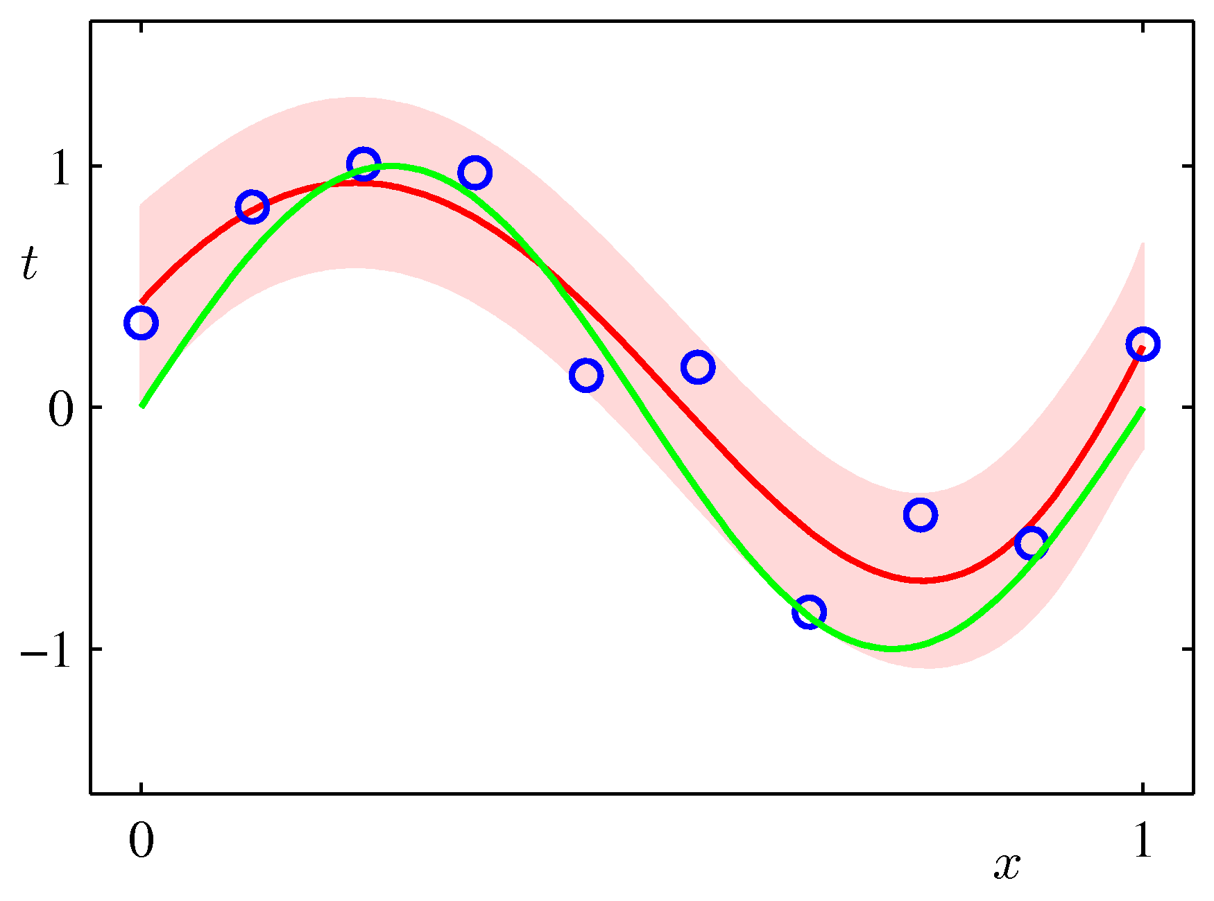 Interpret the height of the band around the most likely function in terms of the distribution of the xs in your synthetic dataset.
Can you think of ways to make this height very small in one segment of the function and large in another?
Interpret the height of the band around the most likely function in terms of the distribution of the xs in your synthetic dataset.
Can you think of ways to make this height very small in one segment of the function and large in another?