ti = y(xi) + Normal(mu, sigma)

where the xi values are equi-distant on the [0,1] segment (that is, x1 = 0, x2=1/N-1, x3=2/N-1..., xN = 1.0)
mu = 0.0
sigma = 0.03
y(x) = sin(2Πx)
Our objective will be to "learn" the function y from the noisy sparse dataset we generate. The function generateDataset(N, f, sigma) should return a tuple with the 2 vectors x and t. Draw the plot (scatterplot) of (x,t) using matplotlib for N=100. Look at the documentation of the numpy.random.normal function in Numpy for an example of usage. Look at the definition of the function numpy.linspace to generate your dataset.
Note: a useful property of Numpy arrays is that you can apply a function to a Numpy array as follows:
import math
import numpy as np
def s(x): return x**2
def f(x): return math.sin(2 * math.pi * x)
vf = np.vectorize(f)        # Create a vectorized version of f

z = np.array([1,2,3,4])

sz = s(z)                   # You can apply simple functions to an array
sz.shape                    # Same dimension as z (4)

fz = vf(z)                  # For more complex ones, you must use the vectorized version of f
fz.shape
y(x) = w0 + w1x + w2x2 + ... + wMxMOur objective is to estimate the vector w = (w0...wM) from the dataset (x, t). We first attempt to solve this regression task by optimizing the square error function (this method is called least squares:
Define: E(w) = 1/2Σi(y(xi) - ti)2
             = 1/2Σi(Σkwkxik - ti)2
If t = (t1, ..., tN), then define the design matrix to be the matrix Φ such that Φnm = xnm = Φm(xn).
We want to minimize the error function, and, therefore, look for a solution to the linear system of equations:
dE/dwk = 0 for k = 0..MWhen we work out the partial derivations, we find that the solution to the following system gives us the optimal value wLS given (x, t):
wLS = (ΦTΦ)-1ΦTt

(Note: Φ is a matrix of dimension Nx(M+1), w is a vector of dimension (M+1) and t is a vector of dimension N.)
Here is how you write this type of matrix operations in Python using the Numpy library:
import numpy as np
import scipy.linalg

t = np.array([1,2,3,4])                    # This is a vector of dim 4
t.shape                                    # (4,)
phi = np.array([[1,1],[2,4],[3,3],[2,4]])  # This is a 4x2 matrix
phi.shape                                  # (4, 2)
prod = np.dot(phi.T, phi)                  # prod is a 2x2 matrix
prod.shape                                 # (2, 2)
i = np.linalg.inv(prod)                    # i is a 2x2 matrix
i.shape                                    # (2, 2)
m = np.dot(i, phi.T)                       # m is a 2x4 matrix
m.shape                                    # (2, 4)
w = np.dot(m, t)                           # w is a vector of dim 2
w.shape                                    # (2,)
Implement a method OptimizeLS(x, t, M) which given the dataset (x, t) returns the optimal polynomial of degree M that approximates the dataset according to the least squares objective. Plot the learned polynomial w*M(xi) and the real function sin(2Πx) for a dataset of size N=10 and M=1,3,5,10.
Define EPLS(w) = E(w) + λEW(w)

Where EPLS is called the penalized least-squares function of w
and   EW is the penalty function.

We will use a standard penalty function:
      EW(w) = 1/2 wT.w = 1/2 Σm=1..Mwm2
When we work out the partial derivatives of the minimization problem, we find in closed form, that the solution to the
penalized least-squares is:
wPLS = (ΦTΦ + λI)-1ΦTtλ is called a hyper-parameter (that is, a parameter which influences the value of the model's parameters w). Its role is to balance the influence of how well the function fits the dataset (as in the least-squares model) and how smooth it is. Write a function optimizePLS(x, t, M, lambda) which returns the optimal parameters wPLS given M and lambda. We want to optimize the value of λ. The way to optimize is to use a development set in addition to our training set. To construct a development set, we will extend our synthetic dataset construction function to return 3 samples: one for training, one for development and one for testing. Write a function generateDataset3(N, f, sigma) which returns 3 pairs of vectors of size N each, (xtest, ttest), (xvalidate, tvalidate) and (xtrain, ttrain). The target values are generated as above with Gaussian noise N(0, sigma). Look at the documentation of the function numpy.random.shuffle() as a way to generate 3 subsets of size N from the list of points generated by linspace. Given the synthetic dataset, optimize for the value of λ by varying the value of log(λ) from -40 to -20 on the development set. Draw the plot of the normalized error of the model for the training, development and test for the case of N = 10 and the case of N=100. The normalized error of the model is defined as:
NEw(x, t) = 1/N [Σi=1..N[ti - Σm=1..Mwmxim]2]1/2Write the function optimizePLS(xt, tt, xv, tv, M) which selects the best value λ given a dataset for training (xt, tt) and a development test (xv, tv). Describe your conclusion from this plot.
tn = y(xn; w) + εnWe now model the distribution of εn as a probabilistic model:
εn ~ N(0, σ2)

since tn = y(xn; w) + εn:

p(tn | xn, w, σ2) = N(y(xn; w), σ2)
We now assume that the observed data points in the dataset are all drawn in an independent manner (iid), we can then express the likelihood of the whole dataset:
p(t | x,w,σ2) = ∏n=1..Np(tn | xn, w, σ2)
              = ∏n=1..N(2Πσ2)-1/2exp[-{tn - y(xn, w)}2 / 2σ2]
We consider this likelihood as a function of the parameters (w and σ) given a dataset (t, x).
If we consider the log-likelihood (which is easier to optimize because we have to derive a sum instead of a product), we get:
-log p(t | w, σ2) = N/2 log(2Πσ2) + 1/2σ2Σn=1..N{tn - y(xn;w)}2
We see that optimizing the log-likelihood of the dataset is equivalent
to minimizing the error function of the least-squares method. That is
to say, the least-squares method is understood as the maximum
likelihood estimator (MLE) of the probabilistic model we just developed, which produces the values wML = wLS.
We can also optimize this model with respect to the second parameter σ2 which, when we work out the derivation and the solution of the equation, yields:
σ2ML = 1/N Σn=1..N{y(xn, wML) - tn}2
Given wML and σ2ML, we can now compute the plugin posterior predictive distribution, which gives us the probability distribution
of the values of t given an input variable x:
p(t | x, wML, σ2ML) = N(t | y(x,wML), σ2ML)This is a richer model than the least-squares model studied above, because it not only estimates the most-likely value t given x, but also the precision of this prediction given the dataset. This precision can be used to construct a confidence interval around t. We further extend the probabilistic model by considering a Bayesian approach to the estimation of this probabilistic model instead of the maximum likelihood estimator (which is known to over-fit the dataset). We choose a prior over the possible values of w which we will, for convenience reasons, select to be of a normal form (this is a conjugate prior as explained in our review of basic probabilities):
p(w | α) = ∏m=0..M(α / 2Π)1/2 exp{-α/2 wm2}
             = N(w | 0, 1/αI)
This prior distribution expresses our degree of belief over the values that w can take.
In this distribution, α plays the role of a hyper-parameter (similar to λ in the regularization model above).
The Bayesian approach consists of applying Bayes rule to the estimation task of the posterior distribution given the dataset:
p(w | t, α, σ2) = likelihood . prior / normalizing-factor
                = p(t | w, σ2)p(w | α) / p(t | α, σ2)
Since we wisely chose a conjugate prior for our distribution over w, we can compute the posterior analytically:
p(w | x, t, α, σ2) = N(μ, Σ)

where Φ is the design matrix as above:

μ = (ΦTΦ + σ2αI)-1ΦTt

Σ = σ2(ΦTΦ + σ2αI)-1
Given this approach, instead of learning a single point estimate of w as in the least-squares and penalized least-squares methods above, we have inferred a distribution over all possible values of w given the dataset. In other words, we have updated our belief about w from the prior (which does not include any information about the dataset) using new information derived from the observed dataset. We can determine w by maximizing the posterior distribution over w given the dataset and the prior belief. This approach is called the maximum posterior (usually written MAP). If we solve the MAP given our selection of the normal conjugate prior, we obtain that the posterior reaches its maximum on the minimum of the following function of w:
1/2σ2Σn=1..N{y(xn, w) - tn}2 + α/2wTw
We find thus that wMAP is in fact the same as the solution of the penalized least-squares method for λ = α σ2.
A fully Bayesian approach, however, does not look for point-estimators of parameters like w. Instead, we are interested in the predictive distribution
p(t | x, x, t). The Bayesian approach consists of marginalizing the predictive distribution over all possible values of the parameters:
p(t | x, x, t) = ∫ p(t|x, w)p(w | x, t) dw(For simplicity, we have hidden the dependency on the hyper-parameters α and σ in this formula.) On this simple case, with a simple normal distribution and normal prior over w, we can solve this integral analytically, and we obtain:
p(t | x, x, t) = N(t | m(x), s2(x))

where the mean and variance are:

m(x) = 1/σ2 Φ(x)TS Σn=1..NΦ(xn)tn

s2(x) = σ2 + Φ(x)TSΦ(x)

S-1 = αI + 1/σ2 Σn=1..NΦ(xn)Φ(xn)T

Φ(x) = (Φ0(x) ... ΦM(x))T = (1 x x2 ... xM)T
Note that the mean and the variance of this predictive distribution depend on x. Your task: write a function bayesianEstimator(x, t, M, alpha, sigma2) which given the dataset (x, t) of size N, and the parameters M, alpha, and sigma2 (the variance), returns a tuple of 2 functions (m(x) var(x)) which are the mean and variance of the predictive distribution inferred from the dataset, based on the parameters and the normal prior over w. As you can see, in the Bayesian approach, we do not learn an optimal value for the parameter w, but instead, marginalize out this parameter and directly learn the predictive distribution. Note that in Python, a function can return a function (like in Scheme) using the following syntax:
def adder(x):
    return lambda(y): x+y

a2 = adder(2)

print(a2(3))       // prints 5
print(adder(4)(3)) // prints 7
Draw the plot of the original function y = sin(2Πx) over the range [0..1], the mean of the predictive distribution m(x) and the confidence interval
(m(x) - var(x)1/2) and (m(x) + var(x)1/2) (that is, one standard deviation around each predicted point) for the values:
alpha = 0.005
sigma2 = 1/11.1
M = 9
over a synthetic dataset of size N=10 and N=100. The plot should look similar to the Figure below (from Bishop p.32).
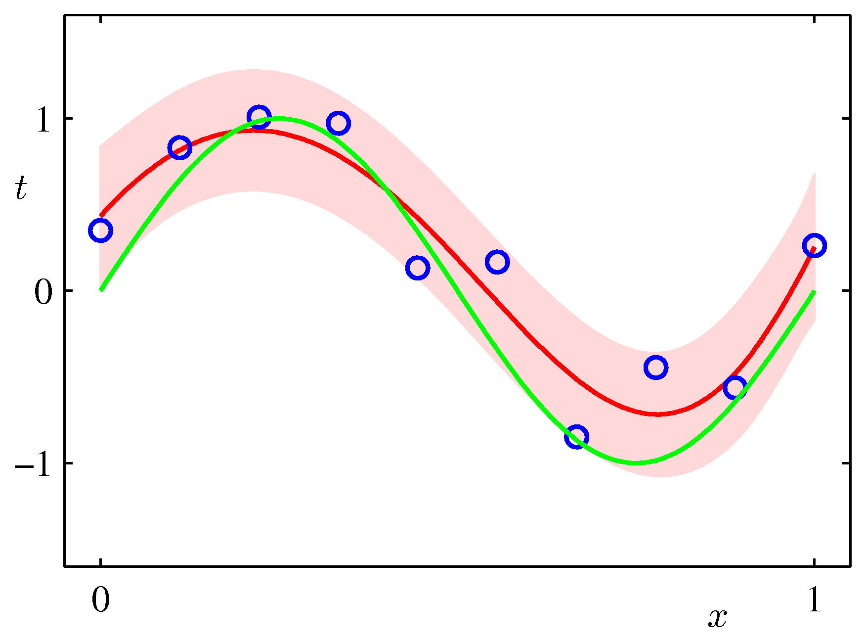 Interpret the height of the band around the most likely function in terms of the distribution of the xs in your synthetic dataset.
Can you think of ways to make this height very small in one segment of the function and large in another?
Interpret the height of the band around the most likely function in terms of the distribution of the xs in your synthetic dataset.
Can you think of ways to make this height very small in one segment of the function and large in another?
Wolff, currently a journalist in Argentina, played with Del Bosque in the final years of the seventies in Real Madrid.

[PER Wolff ] , currently a journalist in [LOC Argentina ] , played with [PER Del Bosque ] in the final years
of the seventies in [ORG Real Madrid ] .
NER involves 2 sub-tasks: identifying the boundaries of such expressions (the open and close brackets) and labelling the expressions (with tags such as PER, LOC or ORG). As for the task of chunking, this sequence labelling task is mapped to a classification tag, using a BIO encoding of the data:
        Wolff B-PER
            , O
    currently O
            a O
   journalist O
           in O
    Argentina B-LOC
            , O
       played O
         with O
          Del B-PER
       Bosque I-PER
           in O
          the O
        final O
        years O
           of O
          the O
    seventies O
           in O
         Real B-ORG
       Madrid I-ORG
            . O
from nltk.corpus import conll2002

etr = conll2002.chunked_sents('esp.train') # In Spanish
eta = conll2002.chunked_sents('esp.testa') # In Spanish
etb = conll2002.chunked_sents('esp.testb') # In Spanish

dtr = conll2002.chunked_sents('ned.train') # In Dutch
dta = conll2002.chunked_sents('ned.testa') # In Dutch
dtb = conll2002.chunked_sents('ned.testb') # In Dutch
The data consists of three files per language (Spanish and Dutch): one training file and two test files testa and testb.
The first test file is to be used in the development phase for finding good parameters for the learning system.
The second test file will be used for the final evaluation.
from nltk.classify import SklearnClassifier
train_data = [({"a": 4, "b": 1, "c": 0}, "ham"),
              ({"a": 5, "b": 2, "c": 1}, "ham"),
              ({"a": 0, "b": 3, "c": 4}, "spam"),
              ({"a": 5, "b": 1, "c": 1}, "ham"),
              ({"a": 1, "b": 4, "c": 3}, "spam")]
test_data = [{"a": 3, "b": 2, "c": 1},
             {"a": 0, "b": 3, "c": 7}]
from sklearn.svm import SVC
classif = SklearnClassifier(SVC(), sparse=False).train(train_data)
classif.classify_many(test_data)
Read about the SVM classifier in the sklearn svm documentation.
The key parameters to optimize when training an SVM classifier are:
classifl = SklearnClassifier(SVC(kernel='linear', C=1.0), sparse=False).train(train_data)
classifr = SklearnClassifier(SVC(kernel='rbf', C=0.5), sparse=False).train(train_data)
from sklearn.svm import LinearSVC
classif_ova = SklearnClassifier(LinearSVC(C=1.0), sparse=False).train(train_data) # LinearSVC() always uses a linear kernel.
You can find code in the Classification notebook that shows how to optimize the C value on a dataset using sklearn methods.
        Wolff NP  B-PER
            , ,   O
    currently RB  O
            a AT  O
   journalist NN  O
           in IN  O
    Argentina NP  B-LOC
            , ,   O
       played VBD O
         with IN  O
          Del NP  B-PER
       Bosque NP  I-PER
           in IN  O
          the AT  O
        final JJ  O
        years NNS O
           of IN  O
          the AT  O
    seventies NNS O
           in IN  O
         Real NP  B-ORG
       Madrid NP  I-ORG
            . .   O

Classes
1 B-PER
2 I-PER
3 B-LOC
4 I-LOC
5 B-ORG
6 I-ORG
7 O

Feature WORD-FORM:
1 Wolff
2 ,
3 currently
4 a
5 journalist
6 in
7 Argentina
8 played
9 with
10 Del
11 Bosque
12 the
13 final
14 years
15 of
16 seventies
17 Real
18 Madrid
19 .

Feature POS
20 NP
21 ,
22 RB
23 AT
24 NN
25 VBD
26 JJ
27 NNS
28 .

Feature ORT
29 number
30 contains-digit
31 contains-hyphen
32 capitalized
33 all-capitals
34 URL
35 punctuation
36 regular

Feature Prefix1
37 W
38 ,
39 c
40 a
41 j
42 i
43 A
44 p
45 w
46 D
47 B
48 t
49 f
50 y
51 o
52 s
53 .
Given this encoding, we can compute the vector representing the first word "Wolff NP B-PER" as:
# Class: B-PER=1
# Word-form: Wolff=1
# POS: NP=20
# ORT: Capitalized=32
# prefix1: W=37
1 1:1 20:1 32:1 37:1
When you encode the test dataset, some of the word-forms will be unknown (not seen in the training dataset). You should, therefore, plan for a special value for each feature of type "unknown" when this is expected. You can either write the code as explained above, or learn to use the Scikit-learn pipeline library - specifically looking at the DictVectorizer class.
from nltk.corpus import reuters

print(reuters.readme())

cats = reuters.categories()
print("Reuters has %d categories:\n%s" % (len(cats), cats))

total = len(reuters.paras())
total_multi = 0
for c in cats:
    lc = len(reuters.paras(categories=[c]))
    total_multi += lc
    print("%s ---- %d documents out of %d" % (c, lc, total))
print("Articles belong to %.4f categories on average" % ((total_multi * 1.0) / total))
print("There are %.4f articles per category on average" % ((total * 1.0) / len(cats)))
As you see, in a few cases, a document belongs to more than one category (on average a
document belongs to 1.2 categories).
reuters.fileids(categories=['yen'])

[u'test/14913',
 u'test/15400',
 u'test/15432',
 u'test/15454',
 ...
 u'training/10364',
 u'training/10679',
 u'training/10681',
 u'training/10684',
 u'training/10689',
 ...]