|
|
|
Course Home |
| Administration |
| Syllabus |
| References |
| Lecture Notes |
| Readings |
| Assignments |
| Lab sessions |
| Student Projects |
| Resources |
|
|
|
Comments? Idea? |
|
|

Automatic Recognition of a Chemestry Atom-Configuration GraphFinal project byAdi Barchan and Kfir Wolfsonbarchan "at" cs.bgu.ac.il, wolfsonk "at" cs.bgu.ac.il1. Introduction
1.1 GoalThe goal of this project is to recognize a given Electron-Configuration Graph, of a chemical matter. These graphs are in extensive use in chemistry studies, laboratories and textbooks. This project helps a Chemistry student to top-up his handwritten electron-configuration drawing abilities, and help her/him recognize different atom drawings.The main problem to tackle is the fact that the drawing is handwritten, and as such not very accurate and grid-aligned. The program also outputs these inaccuracies in the student's drawing. The program could be useful in schools, universities and even at home. Next, we will give a scientific introduction to electron-configuration graphs. . 1.2 Scientific introduction*The electron configuration of an atom is the arrangement of the electrons in its electron orbitals. These are the quantum states of an individual electron in the electron cloud.The orbitals are arranged in sub-shells, we call levels, which are numbered: 1s 2s 2p 3s 3p, etc. [5]: "Additionally, an electron always tries to occupy the lowest possible energy state. It is possible for it to occupy any orbital� but if lower-energy orbitals are available, this condition is unstable. The electron will eventually lose energy (by releasing a photon) and drop into the lower orbital. Thus, electrons fill orbitals in � " a special order. Our graphs are only of stable states. Thus: Due to these limitations, there is a 1-1 correlation between an atom of an element, and a configuration graph (drawing). Our program can thus return the atom of an input drawing. A visual description of electron-spin is the direction in which the electron spins around its axis. There are 2 kinds of spins: up and down, and are marked with the appropriate arrows. In the current version of our program we tried to implement the spin limitation, but the handwritten variety of diagonal lines made it too unpredictable and hard to use. * Summerised from [1] and [5] 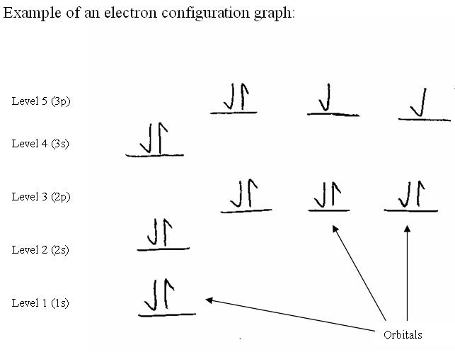
2. Approach and Method
2.1 AlgorithmThe program asks the user to input a 1-bit Bitmap image for analyzing, i.e. a scanned drawing of an electron-configuration graph. Above example is a possible input drawing (made by a somewhat not very accurate student)The following stages are then taken to recognize and interpret every detail in the image. The Computational-Vision algorithms used will be explained in more details in section 3. First, we would like to recognize the level of the atom, i.e. the horizontal lines in the drawing. Stage I - Edge Detection of horizontal lines. Using the Prewitt edge detector, we discover edge points along with the direction of the edge at each point. We then save only the points with a horizontal direction (0 or 180 ). This stage reduces the effect of non-relevant items in the drawing (vertical lines etc.) and noise on the algorithm used in Stage II. Stage II - Horizontal lines detection, using the Hough transform for linear lines. We implemented the transform from the Image Space (x,y) to a Parameter Space (a,b), such that y = ax+b is a line that crosses the point (x,y). More details on the transform in section 3. As we are interested only in horizontal lines, we don't need the "a" (tangent) value of the line, but just the "b" (elevation) value. The transform is applied to the output of Stage I. The following figure shows the original image, with the detected electron levels, i.e. non-adjacent horizontal lines Next, we need to go back to the original image, and discover the exact location of each orbital in the drawing. These are the short horizontal lines in each level, along with the arrows above them. Stage III - Find centers of orbitals, using the K-Clustering algorithm. We first need to segment the image into horizontal stripes, one for each level. According to Chemistry rules, each level has a known number of orbitals, for example the third level from the bottom (marked "2p") has 3 orbitals. This number is used as the "K", or the number of clusters to search for, in the K-Clustering algorithm. We used Matlab's built-in "c clustering" implementation as a black box, for this algorithm. Stage IV - Segment image into small sub-images (of orbitals) Each red circle is an approximation to the center of gravity of an orbital. Taking a rectangular window around each circle, will give us a sub-image, which will hopefully contain only the orbital. For each orbital, we need to detect the amount of electrons. Each vertical arrow above the line represents one electron. Counting vertical arrows is equivalent to counting the number of vertical lines in each sub-image. Stage V - Detect and count vertical lines in each sub image. As we have an algorithm for detecting horizontal lines, all we need to do is rotate by 90 and apply stages I and II, to each sub-image. The number of lines (electrons) detected in each sub-image (orbital) is saved in a simple data structure, a vector, for the next stage. All that is left to do is compare the result vector of the previous stage (the number of electrons in each orbital) to a chemical database. If an exact match is not found, an approximation is made, for the chemical element drawn in the graph. Stage VI - Approximate chemical element and report errors. The approximation is done by calculating the distance between the result vector and the database. The closest element in the DB, and the distance from it, is plotted to the user. This distance represents the difference between the measured drawing and the approximated element: the smaller the distance, the closer the drawing is to this element. The norm for the distance calculation can be changed by the user. 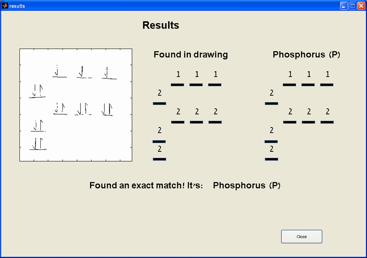
2.2 Logical and Semantic errors in the drawingDuring the run of the algorithm, some student errors in the drawing can be detected. If the error might interfere with the rest of the algorithm (like an incorrect number of levels), then the run is stopped, and the user cannot advance t the next step.The errors detected are in these areas: For Physical reasons of minimal-energy in an atom, the orbitals in a level should be filled with electrons in a left-to-right order, and all orbitals must accommodate an electron before the first one can accommodate two. 2.3 Graphical User Interface (GUI)The GUI takes the user step-by-step in the above algorithm. It asks the user to open a bitmap image, and then stage advancement is triggered by the user clicking a "Next Stage" button.Example Screenshot: 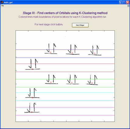
3. Computational Vision AlgorithmsPrewitt Edge DetectionThe Prewitt Edge Detector takes a kernel of the form 1 0 -1 1 0 -1 1 0 -1 and computes a convolution with the input image. In this kernel are both averaging and derivative components. Using it, we compute the Gradient Magnitude and Argument at each pixel. Hough TransformA general transformation from the Image Space (pixels) to a Parameter Space. In our case, the parameter space is (a,b) such that y = ax+b is a line that crosses the point (x,y). The transformation is made in the form of a voting system, where each edge point votes for the lines it may belong to. Lines with the most votes, are probably in the image.K-ClusteringThis algorithm takes a set of points as an input, and divides them into K clusters, with a representative Ci for each cluster. The division of the points is according to a distance function d (Euclidean distance in our case), such that point x is in cluster j if j = argmin{d(x,Ci)}.In each iteration, every point is allocated a certain cluster, and the cluster centers are updated. The algorithm stops when no change has been made. We used the built-in Matlab Fuzzy C-means Clustering function (fcm), which returns a center for each cluster, that doesn't have to be a member of the set of input points. 4. Results & ConclusionsThe main stages of the algorithm work on most inputs. Problems arise in the vertical lines detection. The algorithm does work correctly for input bitmaps with exceptionally strait lines, but fails to identify the correct number of vertical lines in a sub-image for less accurate drawings. This is due to 2 lines being too close, not vertical enough, and other issues arising from the fact that we used the same sensitivity epsilons for different sub-images (orbitals). This may be corrected with per-sub-image sensitivity, in following versions.Drawing errors (like number of levels) in the image are detected correctly by the algorithm. Another problem arises when the arrows are too tall, and so intrude into the image-strip of the above level, thus interfering with the K-Clustering algorithm. The interference is caused by the arrow pixels, which participate in run of the algorithm, as they are part of the set of pixels in the strip. 5.Resources and References[1] Principles of Modern Chemistry; David Oxtoby, HP Gillis, Norman H. Nachtrieb [2] Hypermedia Image Processing Reference, on Roberts Edge Detection [3] Matlab Help and Tutorials [4] ICBV lecture notes [5] Wikipedia [6] Google 6. Additional Information
|